
Table of Contents
Part One
- Introduction
- Abstract
- Background of Linux Commodity Clusters at LLNL
- Commodity Cluster Configurations and Scalable Units
- LC Linux Commodity Cluster Systems
- Intel Xeon Hardware Overview
- Infiniband Interconnect Overview
- Software and Development Environment
- Compilers
- Exercise 1
Or go to Part Two
Introduction
This tutorial is intended to be an introduction to using LC's commodity clusters. In years past, they were sometimes just referred to as Linux clusters or capacity computing clusters. However, with CORAL-2 systems now using TOSS as their OS, all LC systems are Linux systems, and the capacity/capability dichotomy of previous generations has given way to "Commodity Technology Systems" (CTS, as in CTS-1 or CTS-2) and "Advanced Technology Systems" (such as El Capitan and Tuolumne). Throughout the tutorial, the phrase "Linux cluster" may appear—especially in its historical context, but the tutorial itself only covers the technology of the commodity (non-co-designed) systems.
Abstract
This tutorial begins by providing a brief historical background of Linux clusters at LC, noting their success and adoption as a production, high performance computing platform. The primary hardware components of LC's Linux clusters are then presented, including the various types of nodes, processors and switch interconnects. The detailed hardware configuration for each of LC's production commodity clusters completes the hardware related information.
After covering the hardware related topics, software topics are discussed, including the LC development environment, compilers, and how to run both batch and interactive parallel jobs. Important issues in each of these areas are noted. Available debuggers and performance related tools/topics are briefly discussed, however detailed usage is beyond the scope of this tutorial. A lab exercise using one of LC's Linux clusters follows the presentation.
Level/Prerequisites: This tutorial is intended for those who are new to developing parallel programs in LC's commodity cluster environment. A basic understanding of parallel programming in C or Fortran is required. The material covered by the following tutorials would also be helpful:
Background of Linux Commodity Clusters at LLNL
The Linux Project

- LLNL first began experimenting with Linux clusters in 1999-2000 in a partnership with Compaq and Quadrics to port Quadrics software to Alpha Linux.
- The Linux Project was started for several reasons:
- Cost: price-performance analysis demonstrated that near-commodity hardware in clusters running Linux could be more cost-effective than proprietary solutions;
- Focus: the decreasing importance of high-performance computing (HPC) relative to commodity purchases was making it more difficult to convince proprietary systems vendors to implement HPC specific solutions;
- Control: it was believed that by controlling the OS in-house, Livermore Computing could better support its customers;
- Community: the platform created could be leveraged by the general HPC community.
- The objective of this effort was to apply LC's scalable systems strategy (the "Livermore Model") to commodity hardware running the open source Linux OS:
- Based on SMP compute nodes attached to a high-speed, low-latency interconnect.
- Uses OpenMP to exploit SMP parallelism within a node and MPI to exploit parallelism between nodes.
- Provides a POSIX interface parallel filesystem.
- Application toolset: C, C++ and Fortran compilers, scalable MPI/OpenMP GUI debugger, performance analysis tools.
- System management toolset: parallel cluster management tools, resource management, job scheduling, near-real-time accounting.
Alpha Linux Clusters
- The first Linux cluster implemented by LC was LX, a Compaq Alpha Linux system with no high-speed interconnect.
- The first production Alpha cluster targeted to implement the full Livermore Model was Furnace, a 64-node system comprised of dual-CPU EV68 processors with a QSnet interconnect. However...
- Compaq announced the eventual discontinuation of the Alpha server line
- Intel Pentium 4 with favorable SPECfp performance was released just as Furnace was delivered.
- This prompted Livermore to shift to an Intel IA32-based model for its Linux systems in July 2001.
- Furnace's interconnect was allocated to the IA32-based PCR clusters (below) instead. It then operated as a loosely coupled cluster until it was decommissioned in 10/03.
PCR Clusters
- August 2001: The Parallel Capacity Resource (PCR) clusters were purchased from Silicon Graphics and Linux NetworX. Consisted of:
- Adelie: 128-node production cluster
- Emperor: 88-node production cluster
- Dev: 26-node development cluster
- Each PCR compute node had two 1.7-GHz Intel Pentium 4 CPUs and a QsNet Elan3 interconnect.
- Parallel file system was not implemented at that time - instead dedicated BlueArc NFS servers were used.
- SCF resource only
- The 16-node Pengra cluster was procured for the OCF to provide a less restrictive development environment for PCR related work in July, 2002.
- For more information see the: 2002 Linux Project Report.
MCR Cluster...and More

- The success of the PCR clusters was followed by the purchase of the Multiprogrammatic Capability Resource (MCR) cluster in July, 2002 from Linux NetworX.
- 1152 node cluster comprised of dual-processor, 2.4 GHz Intel Xeons
- MCR's procurement was intended to significantly increase the resources available to Multiprogrammatic and Institutional Computing (M&IC) users.
- MCR's configuration included the first production implementation of the Lustre parallel file system, an integral part of the "Livermore Model".
- Debuted as #5 on the Top500 Supercomputers list in November, 2002, and then peaked at #3 in June, 2003.
- For more information see: MCR Background
-
Convinced of the success of this path, LC implemented several other IA-32 Linux clusters simultaneously with, or after, the MCR Linux cluster:
System Network Nodes CPUs/Cores Gflops ALC OCF 960 1,920 9,216 LILAC SCF 768 1,536 9,186 ACE SCF 160 320 1,792 SPHERE OCF 96 192 1,075 GVIZ SCF 64 128 717 ILX OCF 67 134 678 PVC OCF 64 128 614
Which Led To Thunder...
In September, 2003 the RFP for LC's first IA-64 cluster was released. Proposal from California Digital Corporation, a small local company, was accepted.
The Peloton Systems
- In early 2006, LC launched its Opteron/Infiniband Linux cluster procurement with the release of the Peloton RFP.
- Appro was awarded the contract in June, 2006.
- Peloton clusters were built in 5.5 teraflop "scalable units" (SU) of ~144 nodes
- All Peloton clusters used AMD dual-core Socket F Opterons:
- 8 cpus per node
- 2.4 GHz clock
- Option to upgrade to 4-core Opteron "Deerhound" later (not taken)
-
The six Peloton systems represented a mix of resources: OCF, SCF, ASC, M&IC, Capability and Capacity:
System Network Nodes Cores Teraflops Atlas OCF 1,152 9,216 44.2 Minos SCF 864 6,912 33.2 Rhea SCF 576 4,608 22.1 Zeus OCF 288 2,304 11.1 Yana OCF 83 640 3.1 Hopi SCF 76 608 2.9 - The last Peloton clusters were retired in June 2012.
And Then, TLCC and TLCC2
- In July, 2007 the Tri-laboratory Linux Capacity Cluster (TLCC) RFP was released.
- The TLCC procurement represents the first time that the Department of Energy/National Nuclear Security Administration (DOE/NNSA) has awarded a single purchase contract that covers all three national defense laboratories: Los Alamos, Sandia, and Livermore. Read the announcement HERE.
- The TLCC architecture is very similar to the Peloton architecture: Opteron multi-core processors with an Infiniband interconnect. The primary difference is that TLCC clusters are quad-core instead of dual-core.
-
TLCC clusters were/are:
System Network Nodes Cores Teraflops Juno SCF 1,152 18,432 162.2 Hera OCF 864 13,824 127.2 Eos SCF 288 4,608 40.6 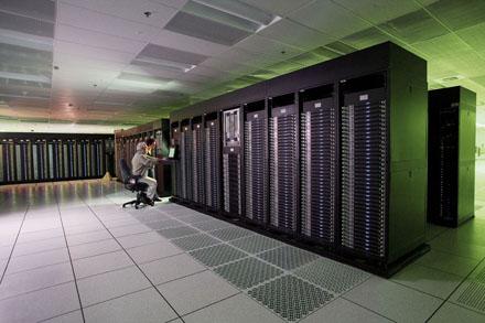
Juno, Eos TLCC Clusters - In June, 2011 the TLCC2 procurement was announced, as a follow-on to the successful TLCC systems. Press releases:
-
The TLCC2 systems consist of multiple Intel Xeon E5-2670 (Sandy Bridge EP), QDR Infiniband based clusters:
System Network Nodes Cores Teraflops Zin SCF 2,916 46,656 961.1 Cab OCF-CZ 1,296 20,736 426.0 Rzmerl OCF-RZ 162 2,592 53.9 Pinot SNSI 162 2,592 53.9 - Additionally, LC procured other Linux clusters similar to TLCC2 systems for various purposes.


Commodity Technology Systems (CTS-1)
- CTS-1 systems are the follow-on to TLCC2 systems.
-
CTS-1 systems became available in late 2016 - early 2017. These systems were based on Intel Broadwell E5-2695 v4 processors, 36 cores per node, 128 GB node memory, with Intel Omni-Path 100 Gb/s interconnect. They included:
System Network Nodes Cores Teraflops Agate SCF 48 1,728 58.1 Borax OCF-CZ 48 1,728 58.1 Jade SCF 2,688 96,768 3,251.4 Mica SCF 384 13,824 530.8 Quartz OCF-CZ 3,072 110,592 3,715.9 RZGenie OCF-RZ 48 1,728 58.1 RZTopaz OCF-RZ 768 27,648 464.5 RZTrona OCF-RZ 20 720 24.2
The CTS-2 Era
The first CTS-2 systems became available in 2022, with major systems Dane and Bengal being deployed in 2023 and becoming Generally Available in 2024.

| Sort descending | Zone | Nodes* | Cores per Node | Memory per Node (GB) | Peak PFLOPS (CPUs) |
|---|---|---|---|---|---|
| Bengal | SCF | 1,158 | 112 | 256 | 7.966 |
| Dane | CZ | 1,544 | 112 | 256 | 10.700 |
| Matrix | CZ | 30 | 112 | 504 | 0.198 |
| Poodle—Decommissioned | CZ | 41 | 112 | 256 | 0.293 |
| RZHound | RZ | 386 | 112 | 256 | 2.655 |
| RZVector | RZ | 16 | 112 | 504 | |
| RZWhippet | RZ | 36 | 112 | 256 | 0.293 |
For more detailed information on the CTS-2 systems, see: https://hpc.llnl.gov/hardware/compute-platforms and search on "class" = CTS-2.
Cluster Configurations and Scalable Units
Basic Components
- Currently, LC has several types of production Linux clusters based on the following processor architectures:
- Intel Xeon 36-core E5-2695 v4
- Intel Xeon 36-core CLX-8276L
- Intel Xeon 112-core Sapphire Rapids
- All of LC's Linux clusters differ in their configuration details, however they do share the same basic hardware building blocks:
- Nodes
- Frames / racks
- High speed interconnect (most clusters)
- Other hardware (file systems, management hardware, etc.)
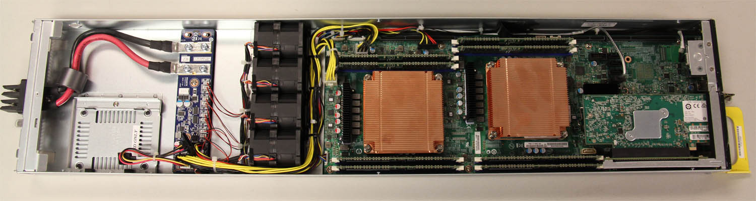
Nodes
- The basic building block of a Linux cluster is the node. A node is essentially an independent computer. Key features:
- Self-contained, diskless, multi-core computer.
- Low form-factor - Clusters nodes are very thin in order to save space.
- Rack Mounted - Nodes are mounted compactly in a drawer fashion to facilitate maintenance, reduced footprint, etc.
- Remote Management - There is no keyboard, mouse, monitor or other device typically used to interact with a computer. All node management occurs over the network from a "management" node.
- Examples (click for larger image):

- In general, an LC production cluster has four types of nodes, based upon function, which can differ in configuration details:
- Login
- Interactive/debug
- Batch
- I/O and service nodes (unavailable to users)
- Login nodes:
- Every system has a designated number of login nodes - depends upon the size of the system. Some examples from decommissioned machines:
- agate = 2
- sierra = 5
- quartz = 14
- zin = 20
- Login nodes are shared by multiple users
- Primarily used for interactive work such as editing files, submitting batch jobs, compiling, running GUIs, etc.
- Interactive use exclusively - login only nodes do not permit any batch jobs.
- DO NOT run production jobs on login nodes! Remember, you are sharing login nodes with other users.
- Every system has a designated number of login nodes - depends upon the size of the system. Some examples from decommissioned machines:
- Interactive/debug (pdebug) nodes:
- Most LC systems have nodes that are designated for interactive work.
- Meant for testing, prototyping, debugging, and small, short jobs
- Cannot be logged into unless you already have a job running on them
- Nodes run one job at a time - not shared like login nodes
- Can also be used through the batch system
- Batch (pbatch) nodes:
- Comprise the majority of nodes on each system
- Meant for production work
- Work is submitted via a batch scheduler (Slurm, Moab)
- Cannot be logged into unless you already have a job running on them
- Nodes run one job at a time - not shared like login nodes
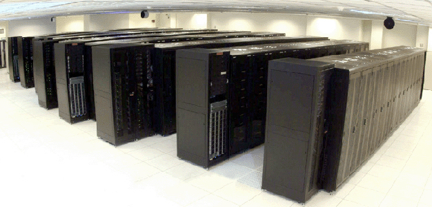
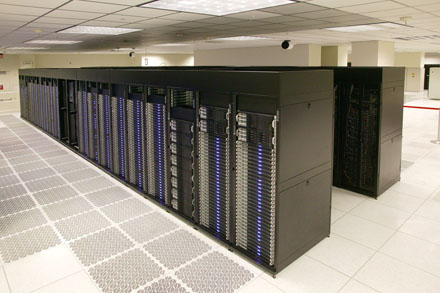
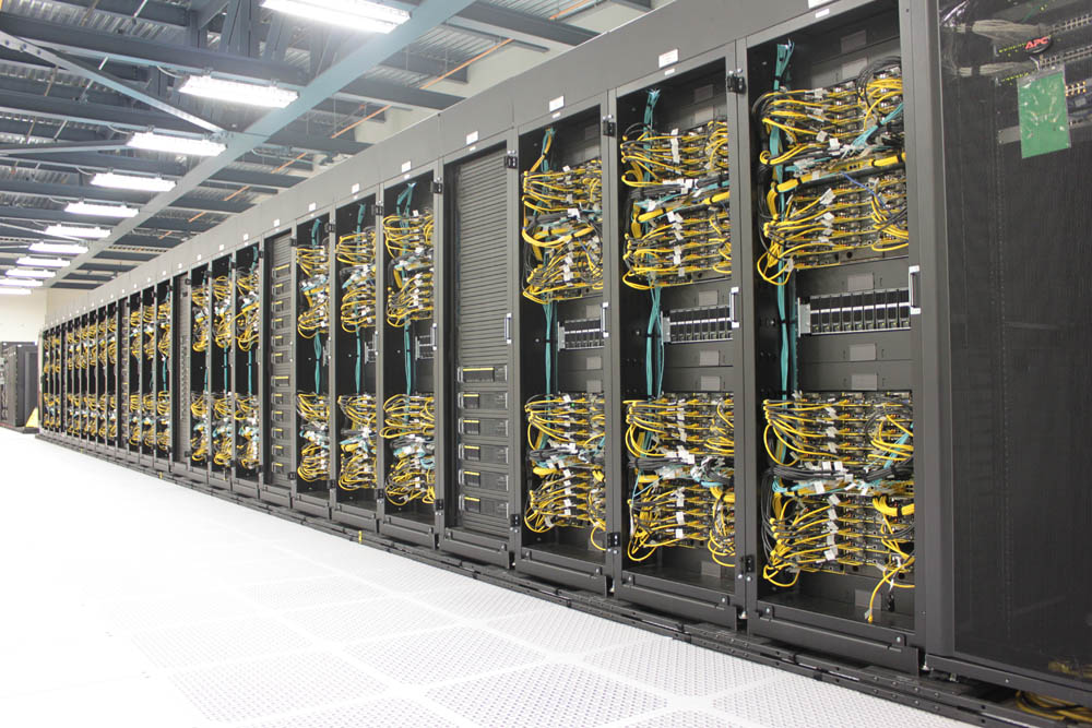
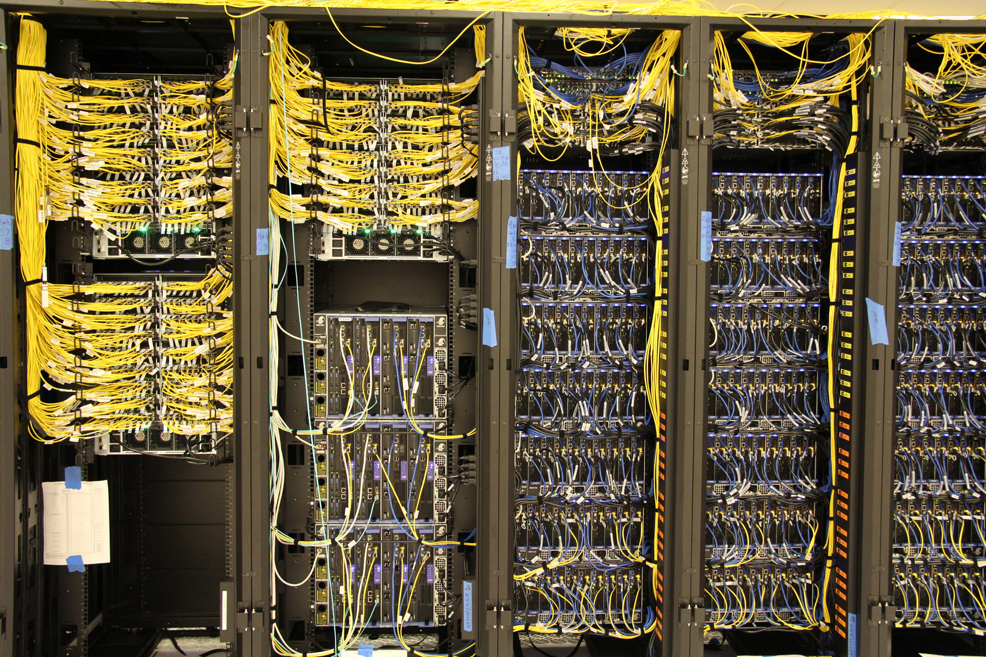
Frames / Racks
- Frames are the physical cabinets that hold most of a cluster's components:
- Nodes of various types
- Switch components
- Other network components
- Parallel file system disk resources (usually in separate racks)
- Vary in size/appearance between the different Linux clusters at LC.
- Power and console management - frames include hardware and software that allow system administrators to perform most tasks remotely.
- Example images below (click for larger image):

Scalable Unit
- The basic building block of LC's production Linux clusters is called a "Scalable Unit" (SU). An SU consists of:
- Nodes (compute, login, management, gateway)
- First stage switches that connect to each node directly
- Miscellaneous management hardware
- Frames sufficient to house all of the hardware
- Additionally, second stage switch hardware is needed to connect multi-SU clusters (not shown).
- The number of nodes in an SU depends upon the type of switch hardware being used. For example:
- QLogic = 162 nodes
- Intel Omni-Path = 192 nodes
- Multiple SUs are combined to create a cluster. For example:
- 2 SU = 324 / 384 nodes
- 4 SU = 648 / 768 nodes
- 8 SU = 1296 / 1536 nodes
- The SU design is meant to:
- Standardize configuration details across the enterprise
- Easily "grow" clusters in incremental units
- Leverage procurements and reduce costs across the Tri-labs
-
An example of a 2 SU cluster is shown below for illustrative purposes. Note that a frame holding the second level switch hardware is not shown.
2 SU Cluster example
LC Linux Commodity Cluster Systems
LC Linux Clusters Summary
- The table below summarizes the key characteristics of LC's Linux commodity clusters.
- Note that some systems are limited access and not Generally Available (GA)
| Sort descending | Zone | Nodes* | Cores per Node | Memory per Node (GB) | Peak PFLOPS (CPUs) |
|---|---|---|---|---|---|
| Bengal | SCF | 1,158 | 112 | 256 | 7.966 |
| Dane | CZ | 1,544 | 112 | 256 | 10.700 |
| Jade | SCF | 1,302 | 36 | 128 | 1.575 |
| Jadeita | SCF | 1,270 | 36 | 128 | 1.536 |
| Magma | SCF | 772 | 96 | 384 | 5.313 |
| Mammoth | CZ | 69 | 128 | 2,048 | 0.294 |
| Matrix | CZ | 30 | 112 | 504 | 0.198 |
| Mica | SCF | 384 | 36 | 128 | 0.464 |
| Pinot | SNSI | 187 | 36 | 128 | 0.232 |
| RZGenie | RZ | 48 | 36 | 128 | 0.058 |
| RZHound | RZ | 386 | 112 | 256 | 2.655 |
| RZVector | RZ | 16 | 112 | 504 | |
| RZWhippet | RZ | 36 | 112 | 256 | 0.293 |
| Tron | SCF | 146 | 32 | 384 | 0.433 |
Intel Xeon Hardware Overview
Intel Xeon Processor
- LC has a long history of Linux clusters using Intel processors.
- Currently, several different types of Xeons are used in LC clusters. Some representative Xeons are discussed below.
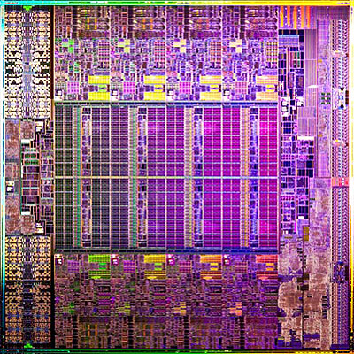
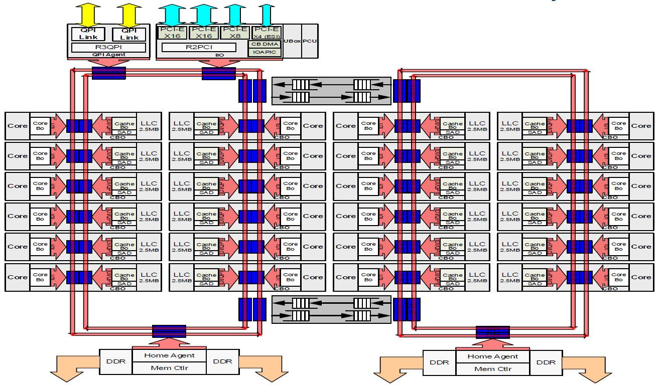
Xeon E5-2670 Processor
- This is the Intel "Sandy Bridge EP" product.
- Used in the Tri-lab TLCC2 clusters
- 64-bit, x86 architecture
- Clockspeed: 2.6 GHz (at LC)
- 8-core (at LC)
- Two threads per core (hyper-threading)
- Cache:
- L1 Data: 32 KB, private
- L1 Instruction: 32 KB, private
- L2: 256 KB, private
- L3: 20 MB, shared
- Memory bandwidth: 51.2 GB/sec
- "Turbo Boost" Technology: automatically allows processor cores to run faster than the base operating frequency if they're operating below power, current, and temperature specification limits. For additional information see: http://www.intel.com/content/www/us/en/architecture-and-technology/turbo-boost/turbo-boost-technology.html.
- Intel AVX (Advanced Vector eXtensions) Instructions:
- New and enhanced instruction set for 256-bit wide vector SIMD operations
- Designed for floating point intensive applications
- Operate on 4 double precision or 8 single precision operands.
- Details: Introduction to Intel Advanced Vector Extensions
- Xeon E5-2670 Spec Sheet

Xeon E5-2695 v4 Processor
- This is the Intel "Broadwell" product.
- Used in the Tri-lab CTS-1 clusters
- 64-bit, x86 architecture
- Clockspeed: 2.1 GHz (at LC)
- 18-core (at LC)
- Two threads per core (hyper-threading)
- Cache:
- L1 Data: 32 KB, private
- L1 Instruction: 32 KB, private
- L2: 256 KB, private
- L3: 45 MB, shared
- Memory bandwidth: 76.8 GB/s
- Turbo Boost Technology
- Intel AVX (Advanced Vector eXtensions) instruction
-
Additional Information
- List / history of Intel processors: en.wikipedia.org/wiki/List_of_Intel_microprocessors
- List / history of Intel Xeon processors: http://en.wikipedia.org/wiki/List_of_Intel_Xeon_microprocessors
- "Sandy Bridge for Servers" by David Kanter: http://realworldtech.com/page.cfm?ArticleID=RWT072811020122
Infiniband Interconnect Overview
Interconnects
- Types of interconnects:
- Varies by cluster; a few clusters do not have interconnects.
- CTS-1 clusters use Intel Omni-Path switches and adapters.
- Most other Intel Xeon clusters use 4x QDR QLogic InfiniBand switches and adapters.
- Bandwidths:
- 4x = 4 times the base InfiniBand link rate of 2.5 Gbits/sec, which equals 10 Gbits/sec, full duplex.
- SDR (Single Data Rate) = 10 Gbits/sec
- DDR (Double Data Rate) = 20 Gbits/sec
- QDR (Quad Data Rate) = 40 Gbits/sec
- Intel Omni-Path = 100 Gbits/sec
Primary components
- Adapter Card:
- Communications processor packaged on network PCI Express adapter card.
- Remote Direct Memory Access (RDMA) improves communication bandwidth by off-loading communications from the CPU.
- Provides the interface between a node and a two-stage network.
- Connected to a first stage switch by copper cable (most cases) or optic fiber.
- Types: Intel Omni-Path, QLogic 4x QDR IB
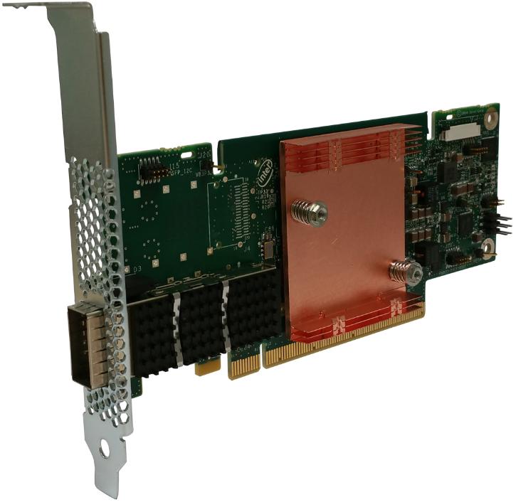
(Image source: Intel)
(Image source: QLogic)
- 1st Stage Switch:
- Intel Omni-Path 48-port: 32 ports connect to adapters in nodes and 16 ports connect to second stage switches.
- QLogic QDR 36-port: 18 ports connect to adapters in nodes and 18 ports connect to second stage switches.
- 2nd Stage Switch:
- Intel Omni-Path 768-port: all used ports connect to a first stage switches via optic fiber cabling.
- QLogic QDR 18-864 port: all used ports connect to a first stage switches via optic fiber cabling.
-
Example image below (click for a larger image):

Example switch
Topology
- Two-stage, federated, bidirectional, fat-tree.
- The number of second stage switches depends upon the number of scalable units (SUs) that comprise the cluster and the type of switch hardware used.
-
Example:
2688-way Interconnect | Quartz/Jade - 14 S
Performance:
-
The inter-node bandwidth measurements below were taken on live, heavily loaded, LC machines using a simple MPI non-blocking test code. One task on each of two nodes. Not all systems are represented. Your mileage may vary.
System Type Latency Bandwidth Intel Xeon Clusters with QDR QLogic ~1-2 us ~4.1 GB/sec Intel Xeon Clusters with QDR QLogic (TLCC2) ~1 us ~5.0 GB/sec Intel Xeon Clusters with Intel Omni-Path (CTS-1) ~1 us ~21 GB/sec
Software and Development Environment
This section only provides a summary of the software and development environment for LC's Linux commodity clusters. Please see the Livermore Computing Resources and Environment tutorial for details.
TOSS Operating System
- All LC Linux clusters use TOSS (Tri-Laboratory Operating System Stack).
- The primary components of TOSS include:
- Red Hat Enterprise Linux (RHEL) distribution with modifications to support targeted HPC hardware and cluster computing
- RHEL kernel optimized for large scale cluster computing
- OpenFabrics Enterprise Distribution InfiniBand software stack including MVAPICH and OpenMPI libraries
- Slurm Workload Manager
- Integrated Lustre and Panasas parallel file system software
- Scalable cluster administration tools
- Cluster monitoring tools
- GNU, C, C++ and Fortran90 compilers (GNU, Intel, PGI)
- Testing software framework for hardware and operating system validation
Batch Systems
- Slurm
- Slurm is the native job scheduling system on each cluster
- SLURM documentation can be found at: http://slurm.schedmd.com/documentation.html
- Moab
- Former workload scheduler for Tri-lab clusters. Now decommissioned.
- Wrapper scripts are available for Moab commands as a convenience.
- Covered in depth in the Slurm and Moab tutorial.
File Systems
- Home directories:
- Globally mounted under /g/g#
- Backed up
- Not purged
- 16 GB quota in effect
- Convenient .snapshot directory for recent backups
- Lustre parallel file systems:
- Mounted under /p/lustre#
- Very large
- Not backed up
- Quota in effect
- Shared by all users on a cluster or multiple clusters
- Lustre is discussed in the Parallel File Systems section of the Introduction to Livermore Computing Resources tutorial.
- Are usually mounted by multiple clusters.
- /usr/workspace - 1 TB NFS file system available for each user and each group. Similar to home directories, but not backed up to tape.
- /var/tmp, /usr/tmp, /tmp - different names for the same file system, local (non-NFS) mounted, moderate size, not backed up, purged, shared by all users on a given node.
- Archival HPSS storage - accessed by ftp storage. Virtually unlimited file space, not backed up or purged. More info: https://hpc.llnl.gov/software/archival-storage-software.
- /usr/gapps - globally mounted project workspace that may be group and/or world readable. More info: hpc.llnl.gov/hardware/file-systems/usr-gapps-file-system.
Modules
- LC's Linux commodity clusters support the Lmod Modules package.
- Provide a convenient, uniform way to select among multiple versions of software installed on LC systems.
- Many LC software applications require that you load a particular "package" in order to use the software.
-
Using Modules:
List available modules:     module avail
Load a module:              module add|load modulefile
Unload a module:            module rm|unload modulefile
List loaded modules:        module list
Read module help info:      module
Display module contents:    module display|show modulefile
- For more information see:
- LC Modules documentation
- TACC documentation: LMOD: ENVIRONMENTAL MODULES SYSTEM
- The module man page
Dotkit
- Dotkit is no longer used on LC production Linux clusters. It has been replaced by Lmod Modules (see above).
Compilers, Tools, Graphics and Other Software
The table below lists and provides links to the majority of software available through LC or related organizations.
| Software Category | Description and More Information |
|---|---|
| Compilers | Lists which compilers are available for each LC system: https://hpc.llnl.gov/software/development-environment-software/compilers |
| Supported Software and Computing Tools | Development Environment Group supported software includes compilers, libraries, debugging, profiling, trace generation/visualization, performance analysis tools, correctness tools, and several utilities: https://hpc.llnl.gov/software/development-environment-software. |
| Graphics Software | Graphics Group supported software includes visualization tools, graphics libraries, and utilities for the plotting and conversion of data: https://hpc.llnl.gov/software/visualization-software |
| Mathematical Software Overview | Lists and describes the primary mathematical libraries and interactive mathematical tools available on LC machines: https://hpc.llnl.gov/software/mathematical-software |
| LINMath | The Livermore Interactive Numerical Mathematical Software Access Utility, is a Web-based access utility for math library software. The LINMath Web site also has pointers to packages available from external sources: https://www-lc.llnl.gov/linmath/ |
| Center for Applied Scientific Computing (CASC) Software | A wide range of software available for download from LLNL's CASC. Includes mathematical software, language tools, PDE software frameworks, visualization, data analysis, program analysis, debugging, and benchmarks: https://software.llnl.gov |
| LLNL Software Portal | Lab-wide portal of software repositories: https://software.llnl.gov/ |
LC Web Services
- LC supports a suite of web-based collaboration tools:
- Confluence: wiki tool, used for documentation, collaboration, knowledge sharing, file sharing, mockups, diagrams... anything you can put on a webpage.
- JIRA: issue tracking and project management system
- GitLab: Git repository hosting, Continuous Integration, Issue tracking
- All three collaboration tools:
- Are based on LC usernames / groups and are intended to foster collaboration between LC users working on HPC projects.
- Are installed on the CZ, RZ and SCF networks
- Require authentication with your LC username and RSA PIN + token
- Have a User Guide for usage information
-
Locations:
Network Confluence Wiki JIRA GitLab CZ https://lc.llnl.gov/confluence/ https://lc.llnl.gov/jira/ lc.llnl.gov/gitlab/ RZ https://rzlc.llnl.gov/confluence/ https://rzlc.llnl.gov/jira/ rzlc.llnl.gov/gitlab/ SCF https://lc.llnl.gov/confluence/ https://lc.llnl.gov/jira/ lc.llnl.gov/gitlab/
Spack
- Spack is a flexible package manager for HPC
-
Easy to download and install. For example:
% . spack/share/spack/setup-env.csh (or setup-env.sh)
- There is an increasing number of software packages (over 3,000 currently) available for installation with Spack. Many open source contributions from the international community.
- To view available packages: spack list
- Then, to install a desired package: spack install packagename
- Additional Spack features:
- Allows installations to be customized. Users can specify the version, build compiler, compile-time options, and cross-compile platform, all on the command line.
- Allows dependencies of a particular installation to be customized extensively.
- Non-destructive installs - Spack installs every unique package/dependency configuration into its own prefix, so new installs will not break existing ones.
- Creation of packages is made easy.
- Extensive documentation is available at: https://spack.readthedocs.io
Compilers
General Information
Available Compilers and Invocation Commands
- The table below summarizes compiler availability and invocation commands on LC Linux clusters.
- Note that parallel compiler commands are actually LC scripts that ultimately invoke the corresponding serial compiler.
-
For details on the MPI parallel compiler commands, see https://hpc-tutorials.llnl.gov/mpi/.
Linux Cluster Compilers Compiler Serial Command Parallel Commands Intel C icc mpicc C++ icpc mpicxx, mpic++ Fortran ifort mpif77, mpif90, mpifort GNU C gcc mpicc C++ g++ mpicxx, mpic++ Fortran gfortran mpif77, mpif90, mpifort PGI C pgcc mpicc C++ pgc++ mpicxx, mpic++ Fortran pgf77, pgf90, pgfortran mpif77, mpif90, mpifort LLVM/Clang C clang mpicc C++ clang++ mpicxx, mpic++
Compiler Versions and Defaults
- LC maintains multiple versions of each compiler.
-
The Modules module avail command is used to list available compilers and versions:
module avail intel module avail gcc module avail pgi module avail clang -
Versions: to determine the actual version you are using, issue the compiler invocation command with its "version" option. For example:
Compiler Option Example Intel --version ifort --version GNU --version g++ --version PGI -V pgf90 -V Clang --version clang --version -
Using an alternate version: issue the Modules command:
module load module-name
Compiler Options
- Each compiler has hundreds of options that determine what the compiler does and how it behaves.
- The options used by one compiler mostly differ from other compilers.
- Additionally, compilers have different default options.
- An in-depth discussion of compiler options is beyond the scope of this tutorial.
- See the compiler's documentation, man pages, and/or -help or --help option for details.
Compiler Documentation
- Intel and PGI: compiler docs are included in the /opt/compilername directory. Otherwise, see Intel or PGI web pages.
- GNU: see the web pages at https://gcc.gnu.org/
- LLVM/Clang: see the web pages at http://clang.llvm.org/docs/
- Man pages may/may not be available
Optimizations
- All compilers are able to perform optimizations, though they will differ between compilers even though the compiler flags appear to be the same.
- Optimizations are intended to make codes run faster, though this isn't guaranteed.
- Some optimizations "rewrite" your code, and can make debugging difficult, since the source may not match the executable.
- Optimizations can also produce wrong results, reduced precision, increased compile times and increased executable size.
-
The table below summarizes common compiler optimization options. See the compiler documentation for details and other optimization options.
Optimization Intel GNU PGI -O Same as O2 Same as O1 O1 + global optimizations. No SIMD. -O0 No optimization DEFAULT. No optimization. Same as omitting any -O flag. No optimization -O1 Optimize for size: basic optimizations to create smallest code Reduce code size and execution time, without performing any optimizations that take a great deal of compilation time. Local optimizations, block scheduling and register allocation. -O2 DEFAULT. Optimize for speed: O1 + additional optimizations such as basic loop and vectorization Optimize even more. O1 + nearly all supported optimizations that do not involve a space-speed tradeoff. -O3 O2 + aggressive loop optimizations. Recommended for loop dominated codes. O2 + further optimizations O2 + aggressive global optimizations -O4 n/a n/a O3 + hoisting of guarded invariant floating point expressions -Ofast Same as O3 (mostly) Same as O3 + optimizations that disregard strict standards compliance. n/a -fast O3 + several additional optimizations n/a Generally specifies global optimization. Actual optimizations vary from release to release. -Og n/a Enables optimizations that do not interfere with debugging. n/a Optimization / Vectorization report -opt-report
-vec-report-ftree-vectorizer-verbose=[1-7]
-ftree-vectorizer-verbose=7-Minfo=[option]
-Minfo=all
Floating-point Exceptions
- The IEEE floating point standard defines several exceptions (FPEs) that occur when the result of a floating point operation is unclear or undesirable:
- overflow: an operation's result is too large to be represented as a float. Can be trapped, or else returned as a +/- infinity.
- underflow: an operation's result is too small to be represented as a normalized float. Can be trapped, or else represented as as a denormalized float (zero exponent w/ non-zero fraction) or zero.
- divide-by-zero: attempting to divide a float by zero. Can be trapped, or else returned as a +/- infinity.
- inexact: result was rounded off. Can be trapped or returned as rounded result.
- invalid: an operation's result is ill-defined, such as 0/0 or the sqrt of a negative number. Can be trapped or returned as NaN (not a number).
- By default, the Xeon processors used at LC mask/ignore FPEs. Programs that encounter FPEs will not terminate abnormally, but instead, will continue execution with the potential of producing wrong results.
- Compilers differ in their ability to handle FPEs. See the relevant compiler documentation for details.
Precision, Performance and IEEE 754 Compliance
- Typically, most compilers do not guarantee IEEE 754 compliance for floating-point arithmetic unless it is explicitly specified by a compiler flag. This is because compiler optimizations are performed at the possible expense of precision.
- Unfortunately for most programs, adhering to IEEE floating-point arithmetic adversely affects performance.
- If you are not sure whether your application needs this, try compiling and running your program both with and without it to evaluate the effects on both performance and precision.
- See the relevant compiler documentation for details.
Mixing C and Fortran
- Modern FORTRAN - FORTRAN 20XX provides much support for interoperability with C/C++ - see the respective compiler documentation.
- If you are linking C/C++ and FORTRAN90/77 code together, and need to explicitly specify the FORTRAN or C/C++ libraries on the link line, LC provides a general recommendation and example in the /usr/local/docs/linux.basics file. See the "MIXING C AND FORTRAN" section.
- All of the other issues involved with mixed language programming apply, such as:
- Column-major vs. row-major array ordering
- Routine name differences - appended underscores
- Arguments passed by reference versus by value
- Common blocks vs. extern structs
- Memory alignment differences
- File I/O - Fortran unit numbers vs. C/C++ file pointers
- C++ name mangling
- Data type differences
- A useful reference:
- Using C/C++ and Fortran Together from http://www.yolinux.com/TUTORIALS/LinuxTutorialMixingFortranAndC.html
Linux Clusters Overview Exercise 1
Getting Started
Overview:
- Login to an LC cluster using your workshop username and OTP token
- Copy the exercise files to your home directory
- Familiarize yourself with the cluster's configuration
- Familiarize yourself with available compilers
- Build and run serial applications
- Compare compiler optimizations