
Table of Contents
Go back to Part One
- Abstract
- Background of Linux Commodity Clusters at LLNL
- Commodity Cluster Configurations and Scalable Units
- LC Linux Commodity Cluster Systems
- Intel Xeon Hardware Overview
- Infiniband Interconnect Overview
- Software and Development Environment
- Compilers
- Exercise 1
On this page, see Part Two
MPI
This section discusses general MPI usage information for LC's Linux commodity clusters. For information on MPI programming, please consult the LC MPI tutorial.
MVAPICH
General Info
- MVAPICH MPI is developed and supported by the Network-Based Computing Lab at Ohio State University.
- Available on all of LC's Linux commodity clusters.
- MVAPICH2
- Default MPI implementation
- Multiple versions available
- MPI-2 and MPI-3 implementations based on MPICH MPI library from Argonne National Laboratory. Versions 1.9 and later implement MPI-3 according to the developer's documentation.
- Thread-safe
-
To see what versions are available, and/or to select an alternate version, use Modules commands. For example:
module avail mvapich         (list available modules)
module load mvapich2/2.3     (use the module of interest)
Compiling
- See the MPI Build Scripts table below.
Running
-
MPI executables are launched using the SLURM srun command with the appropriate options. For example, to launch an 8-process MPI job split across two different nodes in the pdebug pool:
srun -N2 -n8 -ppdebug a.out - The srun command is discussed in detail in the Running Jobs on Linux Clusters section of the Linux Clusters Overview tutorial.
Documentation
- MVAPICH home page: mvapich.cse.ohio-state.edu/
- MVAPICH2 User Guides: http://mvapich.cse.ohio-state.edu/userguide/
Open MPI
General Information
- Open MPI is a thread-safe, open source MPI implementation developed and supported by a consortium of academic, research, and industry partners.
-
Available on all LC Linux commodity clusters. However, you'll need to load the desired Open MPI module first.
module avail openmpi         (list available modules)
module load openmpi/3.0.1    (use the module of interest)
This ensures that LC's MPI wrapper scripts point to the desired version of Open MPI.
Compiling
- See the MPI Build Scripts table below.
Running
- Be sure to load the same Open MPI module that you used to build your executable. If you are running a batch job, you will need to load the module in your batch script.
-
Launching an Open MPI job can be done using the following commands. For example, to run a 48 process MPI job:
mpirun -np 48 a.out
mpiexec -np 48 a.out
srun -n 48 a.out
Documentation
- Open MPI home page: http://www.open-mpi.org/
MPI Build Scripts
- LC developed MPI compiler wrapper scripts are used to compile MPI programs
- Automatically perform some error checks, include the appropriate MPI #include files, link to the necessary MPI libraries, and pass options to the underlying compiler.
Note you may need to load a module for the desired MPI implementation, as discussed previously. Failing to do this will result in getting the default implementation.
-
For additional information:
- See the man page (if it exists)
- Issue the script name with the -help option
- View the script yourself directly
MPI Build Scripts Implementation Language Script Name Underlying Compiler MVAPCH2 C mpicc C compiler for loaded compiler package C++ mpicxx
mpic++C++ compiler for loaded compiler package Fortran mpif77 Fortran77 compiler for loaded compiler package. Points to mpifort. mpif90 Fortran90 compiler for loaded compiler package. Points to mpifort. mpifort Fortran 77/90 compiler for loaded compiler package. Open MPI C mpicc C compiler for loaded compiler package C++ mpiCC
mpic++
mpicxxC++ compiler for loaded compiler package Fortran mpif77 Fortran77 compiler for loaded compiler package. Points to mpifort. mpif90 Fortran90 compiler for loaded compiler package. Points to mpifort. mpifort Fortran 77/90 compiler for loaded compiler package.
Level of Thread Support
- MPI libraries vary in their level of thread support:
- MPI_THREAD_SINGLE - Level 0: Only one thread will execute.
- MPI_THREAD_FUNNELED - Level 1: The process may be multi-threaded, but only the main thread will make MPI calls - all MPI calls are funneled to the main thread.
- MPI_THREAD_SERIALIZED - Level 2: The process may be multi-threaded, and multiple threads may make MPI calls, but only one at a time. That is, calls are not made concurrently from two distinct threads as all MPI calls are serialized.
- MPI_THREAD_MULTIPLE - Level 3: Multiple threads may call MPI with no restrictions.
- Consult the MPI_Init_thread() man page for details.
-
A simple C language example for determining thread level support is shown below.
#include "mpi.h"
#include <stdio.h>

int main( int argc, char *argv[] )
{
    int provided, claimed;

/*** Select one of the following
    MPI_Init_thread( 0, 0, MPI_THREAD_SINGLE, &provided );
    MPI_Init_thread( 0, 0, MPI_THREAD_FUNNELED, &provided );
    MPI_Init_thread( 0, 0, MPI_THREAD_SERIALIZED, &provided );
    MPI_Init_thread( 0, 0, MPI_THREAD_MULTIPLE, &provided );
***/

    MPI_Init_thread(0, 0, MPI_THREAD_MULTIPLE, &provided );
    MPI_Query_thread( &claimed );
        printf( "Query thread level= %d  Init_thread level= %d\n", claimed, provided );

    MPI_Finalize();
}
Sample output:
Query thread level= 3 Init_thread level= 3
Running Jobs
Overview
Big Differences
-
LC's Linux commodity clusters can be divided into two types: those having a high speed intra-node interconnect and those that don't. Those systems without such an interconnect are intended for either serial or parallel applications that can run within one node using either shared-memory, or MPI within that node.
Interconnect No Interconnect Clusters Most linux clusters agate, borax, rztrona Parallelism Designated as a parallel resource.
A single job can span many nodes.Designated for serial and single node parallel jobs only.
A job cannot span more than one node.Node Sharing Compute nodes are NOT shared with other users or jobs.
When your job runs, the allocated nodes are dedicated to your job alone.Multiple users and their jobs can run on the same node simultaneously.
Can result in competition for resources such as CPU and memory. - Usage differences between these two different types of clusters will be noted as relevant in the remainder of this tutorial.
Job Limits
- For all production clusters, there are defined job limits which vary from cluster to cluster. The primary job limits apply to:
- How many nodes/cores a job may use
- How long a job may run
- How many simultaneous jobs can a user run?
- What time of the day/week can jobs run?
- Most job limits are enforced by the batch system.
- Some job limits are enforced by a "good neighbor" policy
-
An easy way to determine the job limits for a machine where you are logged in is to use the command:
news job.lim.machinename
where machinename is the name of the machine you are logged into
- Job limits are also documented on the "MyLC" web pages:
- OCF-CZ: mylc.llnl.gov
- OCF-RZ: rzmylc.llnl.gov
- SCF: https://lc.llnl.gov/lorenz
- Further discussion, and a summary table of job limits for all production machines are available in the Queue Limits section of the Slurm and Moab tutorial.
Batch Versus Interactive
Interactive Jobs (pdebug)
- Most LC clusters have a pdebug partition that permits users to run "interactively" from a login node.
- Your job is launched from the login node command line using the srun command - covered in the Starting Jobs section.
- The job then runs on a pdebug compute node(s) - NOT on the login node
- stdin, stdout, stderr are handled to make it appear the job is running locally on the login node
- Important: As the name pdebug implies, interactive jobs should be short, small debugging jobs, not production runs:
- Shorter time limit
- Fewer number of nodes permitted
- There is usually a "good neighbor" policy in effect - don't monopolize the queue
- Some clusters may have additional partitions permitting interactive jobs.
- Although the pdebug partition is generally associated with interactive use, it can also be used for debugging jobs submitted with a batch script (next).
Batch Jobs (pbatch)
This section only provides a quick summary of batch usage on LC's clusters. For details, see the Slurm and Moab Tutorial.
- Typically, most of a cluster's compute nodes are configured into a pbatch partition.
- The pbatch partition is intended for production work:
- Longer time limits
- Larger number of nodes per job
- Limits enforced by batch system rather than "good neighbor" policy
- The pbatch partition is managed by the workload manager
-
Batch jobs must be submitted in the form of a job control script with the sbatch or msub command. Examples:
sbatch myjobscript
sbatch myjobscript -p ppdebug -A mic
msub myjobscript -t 45:00
msub myjobscript
msub myjobscript -q ppdebug -A mic
msub myjobscript -l walltime=45:00
-
Example Slurm job control script:
#!/bin/tcsh
##### These lines are for Slurm
#SBATCH -N 16
#SBATCH -J parSolve34
#SBATCH -t 2:00:00
#SBATCH -p pbatch
#SBATCH --mail-type=ALL
#SBATCH -A myAccount
#SBATCH -o /p/lustre1/joeuser/par_solve/myjob.out

##### These are shell commands
date
cd /p/lustre1/joeuser/par_solve
##### Launch parallel job using srun
srun -n128 a.out
echo 'Done'
- After successfully submitting a job, you may then check its progress and interact with it (hold, release, alter, terminate) by means of other batch commands - discussed in the Interacting With Jobs section.
- Some clusters have additional partitions permitting batch jobs.
- Interactive use of pbatch nodes is facilitated by using the mxterm command.
- Interactive debugging of batch jobs is possible - covered in the Debuggers section.
Starting Jobs - srun
The srun command
- The SLURM srun command is an application task launcher utility for launching parallel jobs (MPI-based, shared-memory and hybrid) - both batch and interactive.
- It should also be used to launch serial jobs in the pdebug and other interactive queues.
-
Syntax:
srun [option list] [executable] [args]
Note that srun options must precede your executable.
-
Interactive use example, from the login node command line. Specifies 2 nodes (-N), 16 tasks (-n) and the interactive pdebug partition (-p):
% srun -N2 -n16 -ppdebug myexe
-
Batch use example requesting 16 nodes and 256 tasks (assumes nodes have 16 cores): First create a job script that requests nodes via #SBATCH -N and uses srun to specify the number of tasks and launch the job.
#!/bin/csh
#SBATCH -N 16
#SBATCH -t 2:00:00
#SBATCH -p pbatch

# Run info and srun job launch
cd /p/lustre1/joeuser/par_solve
srun -n256 a.out
echo 'Done'
Then submit the job script from the login node command line:
% sbatch myjobscript
-
Primary differences between batch and interactive usage:
Difference Interactive Batch Where used: From login node command line In batch script Partition: Requires specification of an interactive partition, such as pdebug with the -p flag pbatch is default Scheduling: If there are available interactive nodes, job will run immediately. Otherwise, it will queue up (fifo) and wait until there are enough free nodes to run it. The batch scheduler handles when to run your job regardless of the number of nodes available. -
More Examples:
srun -n64 -ppdebug my_app
64 process job run interactively in pdebug partition srun -N64 -n512 my_threaded_app
512 process job using 64 nodes. Assumes pbatch partition. srun -N4 -n32 -c2 my_threaded_app
2 node, 32 process job with 2 cores (threads) per process. Assumes pbatch partition. srun -N8 my_app
8 node job with a default value of one task per node (8 tasks). Assumes pbatch partition. srun -n128 -o my_app.out my_app
128 process job that redirects stdout to file my_app.out. Assumes pbatch partition. srun -n32 -ppdebug -i my.inp my_app
32 process interactive job; each process accepts input from a file called my.inp instead of stdin -
Behavior of srun -N and -n flags - using 4 nodes in batch (#MSUB -l nodes=4), each of which has 16 cores:
srun diagram
srun options
- srun is a powerful command with @100 options affecting a wide range of job parameters.
- Many srun options may be set via @60 SLURM environment variables. For example, SLURM_NNODES behaves like the -N option.
-
A short list of common srun options appears below. srun man page for details on options and environment variables.
Option Description --auto-affinity=[args]
Specifies how to bind tasks to CPUs. See also: auto affinity details. -c [#cpus/task]
The number of CPUs used by each process. Use this option if each process in your code spawns multiple POSIX or OpenMP threads. -d
Specify a debug level - integer value between 0 and 5 -i [file] -o [file]
Redirect input/output to file specified -I
Allocate CPUs immediately or fail. By default, srun blocks until resources become available. -J
Specify a name for the job -l
Label - prepend task number to lines of stdout/err -m block|cyclic
Specifies whether to use block (the default) or cyclic distribution of processes over nodes --multi-prog config_file
Run a job with different programs with/without different arguments for each task. Intended for MPMD (multiple program multiple data) model MPI programs. See more srun --multi-prog information here. -n [#processes]
Number of processes that the job requires -N [#nodes]
Number of nodes on which to run job -O
Overcommit - srun will refuse to allocate more than one process per CPU unless this option is also specified -p [partition]
Specify a partition (cluster) on which to run job -s
Print usage stats as job exits -v -vv -vvv
Increasing levels of verbosity -V
Display version information
Clusters Without an Interconnect - Additional Notes
- The agate, borax and rztrona clusters fall into this category.
- Don't forget that multiple users and jobs can run on a single node
- Important: Please see the "Running on Serial Clusters" section of the Slurm and Moab tutorial for further discussion on running jobs on these clusters.
Interacting With Jobs
This section only provides a quick summary of commands used to interact with jobs. For additional information, see the Slurm and Moab tutorial.
Monitoring Jobs and Displaying Job Information
- There are several different job monitoring commands. Some are based on Moab, some on Slurm, and some on other sources.
-
The more commonly used job monitoring commands are summarized in the table below with links to additional information and examples.
Command Description squeue Displays one line of information per job by default. Numerous options. showq Displays one line of information per job. Similar to squeue. Several options. mdiag -j Displays one line of information per job. Similar to squeue. mjstat Summarizes queue usage and displays one line of information for active jobs. checkjob jobid Provides detailed information about a specific job. sprio -l
mdiag -p -vDisplays a list of queued jobs, their priority, and the primary factors used to calculate job priority. sview Provides a graphical view of a cluster and all job information. sinfo Displays state information about a cluster's queues and nodes
Holding / Releasing Jobs
- Jobs can be placed "on hold" when they are submitted.
- They can also be placed on hold while they are waiting to run.
- Held jobs can then be released to run later
-
More information/examples: see Holding and Releasing Jobs in the Slurm and Moab tutorial.
Command Description sbatch -H jobscript
msub -h jobscriptPut job on hold when it is submitted scontrol hole jobid
mjobctl -h jobidPlace a specific idle jobid on hold scontrol release jobid
mjobctl -u jobidRelease a specific held jobid
Modifying Jobs
- After a job has been submitted, certain attributes may be modified using the scontrol update and mjobctl -m commands.
- Examples of parameters that can be changed: account, queue, job name, wall clock limit...
- More information/examples: see Changing Job Parameters in the Slurm and Moab tutorial.
Terminating / Canceling Jobs
- Interactive srun jobs launched from the command line should normally be terminated with a SIGINT (CTRL-C):
- The first CTRL-C will report the state of the tasks
- A second CTRL-C within one second will terminate the tasks
- For batch jobs, the mjobctl -c and canceljob commands can be used.
- More information/examples: see Canceling Jobs in the Slurm and Moab tutorial.
Optimizing CPU Usage
Clusters with an Interconnect
- Fully utilizing the cores on a node requires that you use the right combination of srun and Slurm/Moab options, depending upon what you want to do and which type of machine you are using.
-
MPI only: for example, if you are running on a cluster that has 16 cores per node, and you want your job to use all 16 cores on 4 nodes (16 MPI tasks per node), then you would do something like:
Interactive Slurm Batch Moab Batch srun -n64 -ppdebug a.out
#SBATCH -N 4
srun -n64 a.out
#MSUB -l nodes=4
srun -n64 a.out
-
MPI with Threads: If your MPI job uses POSIX or OpenMP threads within each node, you will need to calculate how many cores will be required in addition to the number of tasks. For example, running on a cluster having 16 cores per node, an 8-task job where each task creates 4 OpenMP threads, would need a total of 32 cores, or 2 nodes:
8 tasks * 4 threads / 16 cores/node = 2 nodesInteractive Slurm Batch Moab Batch srun -N2 -n8 -ppdebug a.out
#SBATCH -N 2
srun -N2 -n8 a.out
#MSUB -l nodes=2
srun -N2 -n8 a.out
-
You can include multiple srun commands within your batch job command script. For example, suppose that you were conducting a scalability run on a 16-core/node Linux cluster. You could allocate the maximum number of nodes that you would use with #MSUB -l nodes= and then have a series of srun commands that use varying numbers of nodes:
#MSUB -l nodes=8

srun -N1 -n16 myjob
srun -N2 -n32 myjob
srun -N3 -n48 myjob
....
srun -N8 -n128 myjob
Clusters Without an Interconnect
- The issues for CPU utilization are different for clusters without a switch for several reasons:
- Jobs can be serial
- Nodes may be shared with other users
- Heavy utilization
- Jobs are limited to one node
- On these systems, the more important issue is over utilization of cores rather than under utilization.
- Important notes for Agate, Borax and RZTrona users: Please see the "Running on Serial Clusters" section of the Slurm and Moab tutorial for important information about running MPI jobs on these clusters.
Memory Considerations
64-bit Architecture Memory Limit
- Because LC's Linux commodity clusters employ a 64-bit architecture, 16 exabytes of memory can be addressed - which is about 4 billion times more than 4 GB limit of 32-bit architectures. By current standards, this is virtually unlimited memory.
- In reality, systems are usually configured with only GBs of memory, so any address access that exceeds physical memory will result (on most systems) with paging and degraded performance.
- However, most LC commodity cluster systems are an exception to this because they have no local disk - see below.
LC's Diskless Linux Clusters
- Most LC's Linux commodity clusters are configured with diskless compute nodes. This has very important implications for programs that exceed physical memory. For example, most compute nodes have 16-64 GB of physical memory.
- Because compute nodes don't have disks, there is no virtual (swap) memory, which means there is no paging. Programs that exceed physical memory will terminate with an OOM (out of memory) error and/or segmentation fault.
Compiler, Shell, Pthreads and OpenMP Limits
- Compiler data structure limits are in effect, but may be handled differently by different compilers.
- Shell stack limits: most are set to "unlimited" by default.
- Pthreads stack limits apply, and may differ between compilers.
- OpenMP stack limits apply, and may differ between compilers.
MPI Memory Use
- All MPI implementations require additional memory use. This varies between MPI implementations and between versions of any given implementation.
- The amount of memory used increases with the number of MPI tasks.
- Determining how much memory the MPI library uses can be accomplished by using various tools, such as TotalView's Memscape feature.
Large Static Data
- If your executable contains a large amount of static data, LC recommends that you compile with the -mcmodel=medium option.
- This flag allows the Data and .BSS sections of your executable to extend beyond a default 2 GB limit.
- True for all compilers (see the respective compiler man page).
Vectorization and Hyper-threading
Vectorization
- Historically, the Xeon architecture has provided support for SIMD (Single Instruction Multiple Data) vector instructions through Intel's Streaming SIMD Extensions (SSE, SSE2, SSE3, SSE4) instruction sets.
- AVX - Advanced Vector Extension instruction set (2011) improved on SSE instructions by increasing the size of the vector registers from 128-bits to 256-bits. AVX2 (2013) offered further improvements, such as fused multiply-add (FMA) instructions to double FLOPS.
-
The primary purpose of these instructions is to increase CPU throughput by performing operations on vectors of data elements, rather than on single data elements. For example:
Instruction Set Single-precision
Flops/ClockDouble-precision
Flops/ClockSSE4 8 4 AVX 16 8 AVX2 32 16 - Sandy Bridge-EP (TLCC2) processors support SSE and AVX instructions.
- Broadwell (CTS-1) processors support SSE, AVX and AVX2.
-
To take advantage of the potential performance improvements offered by vectorization, all you need to do is compile with the appropriate compiler flags. Some recommendations are shown in the table below.
Compiler SSE Flag AVX Flag Reporting Intel -vec (default)
-axAVX
-axCORE-AVX2
-qopt_report
PGI -Mvect=simd:128
-Mvect=simd:256
-Minfo=all
GNU -O3
-mavx
-mavx2
-fopt-info-all
- Vectorization is performed on eligible loops. Note that not all loops are able to be vectorized. A number of factors can prevent the compiler from vectorizing a loop, such as:
- Function calls
- I/O operations
- GOTOs in or out of the loop
- Recurrences
- Data dependence, such as needing a value from a previous loop iteration
- Complex coding (difficult loop analysis)
-
To view/confirm that a loop has been vectorized, use one of the reporting flags shown above. You can also generate an assembler file and look at the instructions used. For example:
%icc -S -axAVX myprog.c

% cat myprog.s
...
...
.L8:
	movdqa	%xmm3, %xmm1
.L3:
	movdqa	%xmm1, %xmm3
	cvtdq2pd	%xmm1, %xmm0
	pshufd	$238, %xmm1, %xmm1
	addpd	%xmm2, %xmm0
	paddd	%xmm6, %xmm3
	cvtdq2pd	%xmm1, %xmm1
	addpd	%xmm2, %xmm1
	cvtpd2ps	%xmm0, %xmm0
	cvtpd2ps	%xmm1, %xmm1
	movlhps	%xmm1, %xmm0
	movaps	%xmm4, %xmm1
	movaps	%xmm0, (%rcx,%rax)
	mulps	%xmm5, %xmm0
	divps	%xmm0, %xmm1
	movaps	%xmm0, (%rdx,%rax)
	movaps	%xmm1, (%rsi,%rax)
	addq	$16, %rax
	cmpq	$400, %rax
	jne	.L8
	xorl	%eax, %eax
...
...
- Most of the instructions shown above are SIMD instructions using the SIMD xmm registers. For a listing of SSE and AVX instructions, see en.wikipedia.org/wiki/X86_instruction_listings#SIMD_instructions
- More information:
- See your compiler's documentation and/or man page for vectorization options.
- "Streaming SIMD Extensions" at https://en.wikipedia.org/wiki/Streaming_SIMD_Extensions
- "Advanced Vector Instructions" at https://en.wikipedia.org/wiki/Advanced_Vector_Extensions
Hyper-threading
- On Intel processors, hyper-threading enables 2 hardware threads per core.
- Hyper-threading benefits some codes more than others. Tests performed on some LC codes (pF3D, IMC, Ares) showed improvements in the 10-30% range. Application performance can be expected to vary.
- On TOSS 3 systems, hyper-threading is turned on by default. Details are available at: https://lc.llnl.gov/confluence/display/TCE/Hyper-Threading (authentication required).
Process and Thread Binding
Process/Thread Binding to Cores
-
By default, jobs run on LC's Linux clusters have their processes bound to the available cores on a node. For example:
% srun -l -n2 numactl -s | grep physc | sort
0: physcpubind: 0 1 2 3 4 5 6 7
1: physcpubind: 8 9 10 11 12 13 14 15

% srun -l -n4 numactl -s | grep physc | sort
0: physcpubind: 0 1 2 3
1: physcpubind: 4 5 6 7
2: physcpubind: 8 9 10 11
3: physcpubind: 12 13 14 15

% srun -l -n8 numactl -s | grep physc |sort
0: physcpubind: 0 1
1: physcpubind: 2 3
2: physcpubind: 4 5
3: physcpubind: 6 7
4: physcpubind: 8 9
5: physcpubind: 10 11
6: physcpubind: 12 13
7: physcpubind: 14 15
- Binding processes to cores may improve performance by keeping in-cache data local to cores.
- If a process is multi-threaded (such as with OpenMP), the threads will run on any of the cores bound to their process.
- To bind an OpenMP thread to a single core, the OMP_PROC_BIND environment variable can be used (set to "TRUE").
-
Additionally, LC provides a couple useful utilities for binding processes and threads to cores:
mpibind - automatically binds processes and threads to cores. Documentation at https://lc.llnl.gov/confluence/display/LC/mpibind (requires authentication)
mpifind - reports on how processes and threads are bound to cores.
Example output for a 4-process job, each with 4 threads. Output on the left is with OMP_PROC_BIND unset, and on the right, with OMP_PROC_BIND=TRUE.OMP_PROC_BIND unset OMP_PROC_BIND=TRUE cab690% mpifind 777601 HOST RANK ID LCPU AFFINITY CPUMASK CMD cab24 0 98152 3 0-3 0000000f a.out 98160 2 0-3 0000000f a.out 98163 1 0-3 0000000f a.out 98166 0 0-3 0000000f a.out 98173 2 0-3 0000000f a.out cab24 1 98153 7 4-7 000000f0 a.out 98159 4 4-7 000000f0 a.out 98161 5 4-7 000000f0 a.out 98165 6 4-7 000000f0 a.out 98171 4 4-7 000000f0 a.out cab24 2 98154 11 8-11 00000f00 a.out 98162 8 8-11 00000f00 a.out 98167 9 8-11 00000f00 a.out 98170 10 8-11 00000f00 a.out 98174 8 8-11 00000f00 a.out cab24 3 98155 15 12-15 0000f000 a.out 98164 12 12-15 0000f000 a.out 98168 13 12-15 0000f000 a.out 98169 14 12-15 0000f000 a.out 98172 12 12-15 0000f000 a.outcab690% mpifind 777571 HOST RANK ID LCPU AFFINITY CPUMASK CMD cab28 0 151874 0 0 00000001 a.out 151881 0 0-3 0000000f a.out 151883 1 1 00000002 a.out 151886 2 2 00000004 a.out 151892 3 3 00000008 a.out cab28 1 151875 4 4 00000010 a.out 151882 5 4-7 000000f0 a.out 151884 5 5 00000020 a.out 151885 6 6 00000040 a.out 151887 7 7 00000080 a.out cab28 2 151876 8 8 00000100 a.out 151888 9 8-11 00000f00 a.out 151890 9 9 00000200 a.out 151893 10 10 00000400 a.out 151896 11 11 00000800 a.out cab28 3 151877 12 12 00001000 a.out 151889 13 12-15 0000f000 a.out 151891 13 13 00002000 a.out 151894 14 14 00004000 a.out 151895 15 15 00008000 a.out
Debugging
This section only touches on selected highlights. For more information users will want to consult the relevant documentation mentioned below. Also, please see the Development Environment Software web page located at hpc.llnl.gov/software/development-environment-software.
TotalView
- TotalView is probably the most widely used debugger for parallel programs. It can be used with C/C++ and Fortran programs and supports all common forms of parallelism, including pthreads, openMP, MPI, accelerators and GPUs.
- Starting TotalView for serial codes: simply issue the command:
- totalview myprog
- Starting TotalView for interactive parallel jobs:
-
Some special command line options are required to run a parallel job through TotalView under SLURM. You need to run srun under TotalView, and then specify the -a flag followed by 1)srun options, 2)your program, and 3)your program flags (in that order). The general syntax is:
totalview srun -a -n #processes -p pdebug myprog [prog args]
- To debug an already running interactive parallel job, simply issue the totalview command and then attach to the srun process that started the job.
- Debugging batch jobs is covered in LC's TotalView tutorial and in the "Debugging in Batch" section below.
-
- Documentation:
- LC Tutorial: hpc.llnl.gov/documentation/tutorials/totalview-tutorial
- Vendor website: http://www.roguewave.com/
DDT
- DDT stands for "Distributed Debugging Tool", a product of Allinea Software Ltd.
- DDT is a comprehensive graphical debugger designed specifically for debugging complex parallel codes. It is supported on a variety of platforms for C/C++ and Fortran. It is able to be used to debug multi-process MPI programs, and multi-threaded programs, including OpenMP.
- Currently, LC has a limited number of fixed and floating licenses for OCF and SCF Linux machines.
- Usage information: see LC's DDT Quick Start information located at: https://hpc.llnl.gov/software/development-environment-software/allinea-…
- Documentation:
- Vendor website: http://www.allinea.com
- Local copies of documentation under /usr/local/docs/ddt
STAT - Stack Trace Analysis Tool
- The Stack Trace Analysis Tool (developed at LC) gathers and merges stack traces from a parallel application's processes.
- STAT is particularly useful for debugging hung programs.
- It produces call graphs: 2D spatial and 3D spatial-temporal
- The 2D spatial call prefix tree represents a single snapshot of the entire application (see image).
- The 3D spatial-temporal call prefix tree represents a series of snapshots from the application taken over time.
- In these graphs, the nodes are labeled by function names. The directed edges, showing the calling sequence from caller to callee, are labeled by the set of tasks that follow that call path. Nodes that are visited by the same set of tasks are assigned the same color, giving a visual reference to the various equivalence classes.
- This tool should be in your default path as:
- /usr/local/bin/stat-gui - GUI
- /usr/local/bin/stat-cl - command line
- /usr/local/bin/stat-view - viewer for DOT format output files
- /usr/local/tools/stat - install directory, documentation
- More information: see the STAT web page at: hpc.llnl.gov/software/development-environment-software/stat-stack-trace-analysis-tool and the STAT man page.
Other Debuggers
- Several other common debuggers are available on LC Linux clusters, though they are not recommended for parallel programs when compared to TotalView and DDT.
- PGDBG: the Portland Group Compiler debugger. Documentation: https://www.pgroup.com/products/pgdbg.htm
- GDB: GNU GDB debugger, a command-line, text-based, single process debugger. Documentation: http://www.gnu.org/software/gdb
- DDD: GNU DDD debugger is a graphical front-end for command-line debuggers such as GDB, DBX, WDB, Ladebug, JDB, XDB, the Perl debugger, the bash debugger, or the Python debugger. Documentation: http://www.gnu.org/software/ddd
Debugging in Batch: mxterm
- Debugging batch parallel jobs on LC production clusters is fairly straightforward. The main idea is that you need to submit a batch job that gets your partition allocated and running.
- Once you have your partition, you can login to any of the nodes within it, and then starting running as though you’re in the interactive pdebug partition.
- For convenience, LC has developed a utility called mxterm which makes the process even easier.
- How to use mxterm:
- If you are on a Windows PC, start your X11 application (such as X-Win32)
- Make sure you enable X11 tunneling for your ssh session
- ssh and login to your cluster
-
Issue the command as follows:
mxterm #nodes #tasks #minutes
Where:
#nodes = number of nodes your job requires
#tasks = number of tasks your job requires
#minutes = how long you need to keep your partition for debugging - This will submit a batch job for you that will open an xterm when it starts to run.
- After the xterm appears, cd to the directory with your source code and begin your debug session.
- This utility does not have a man page; however, you can view the usage information by simple typing the name of the command.
Core Files
- It is quite likely that your shell's core file size setting may limit the size of a core file so that it is inadequate for debugging, especially with TotalView.
-
To check your shell's limit settings, use either the limit (csh/tcsh) or ulimit -a (sh/ksh/bash) command. For example:
% limit
cputime      unlimited
filesize     unlimited
datasize     unlimited
stacksize    unlimited
coredumpsize 16 kbytes
memoryuse    unlimited
vmemoryuse   unlimited
descriptors  1024
memorylocked 7168 kbytes
maxproc      1024

$ ulimit -a
address space limit (kbytes)   (-M)  unlimited
core file size (blocks)        (-c)  32
cpu time (seconds)             (-t)  unlimited
data size (kbytes)             (-d)  unlimited
file size (blocks)             (-f)  unlimited
locks                          (-L)  unlimited
locked address space (kbytes)  (-l)  7168
nofile                         (-n)  1024
nproc                          (-u)  1024
pipe buffer size (bytes)       (-p)  4096
resident set size (kbytes)     (-m)  unlimited
socket buffer size (bytes)     (-b)  4096
stack size (kbytes)            (-s)  unlimited
threads                        (-T)  not supported
process size (kbytes)          (-v)  unlimited
-
To override your default core file size setting, use one of the following commands:
csh/tcsh unlimit -or- limit coredumpsize 64
sh/ksh/bash ulimit -c 64
- Some users have complained that for many-process jobs, they actually don't want core files or only want small core files because normal core files can fill up their disk space. The limit (csh/tcsh) or ulimit -c (sh/ksh/bash) commands can be used as shown above to set smaller / zero sizes.
A Few Additional Useful Debugging Hints
- Add the sinfo and squeue commands to your batch scripts to assist in diagnosing problems. In particular, these commands will document which nodes your job is using.
- Also add the -l option to your srun command so that output statements are prepended with the task number that created them.
- Be sure to check the exit status of all I/O operations when reading or writing files in Lustre. This will allow you to detect any I/O problems with the underlying OST servers.
-
If you know/suspect that there are problems with particular nodes, you can use the srun -x option to skip these nodes. For example:
srun -N12 -x "cab40 cab41" -ppdebug myjob
Application Development Tools
We Need a Book!
- The subject of "Tools" for Linux cluster applications is far too broad and deep to cover here. Instead, a few pointers are being provided for those who are interested in further research.
- The first place to check are LC's Software web pages at: hpc.llnl.gov/software for what may be available here. Some example tools are listed below.
Memory Correctness Tools
-
Memcheck
-
Valgrind's Memcheck tool detects a comprehensive set of memory errors, including reads and writes of unallocated or freed memory and memory leaks.
-
TotalView
-
Allows you to stop execution when heap API problems occur, list memory leaks, paint allocated and deallocated blocks, identify dangling pointers, hold onto deallocated memory, graphically browse the heap, identify the source line and stack backtrace of an allocation or deallocation, summarize heap use by routine, filter and dump heap information, and review memory usage by process or by library.
-
memP
-
The memP tool provides heap profiling through the generation of two reports: a summary of the heap high-water-mark across all processes in a parallel job as well as a detailed task-specific report that provides a snapshot of the heap memory currently in use, including the amount allocated at specific call sites.
-
Intel Inspector
-
Primarily a thread correctness tool, but memory debugging features are included.
Profiling, Tracing and Performance Analysis
Open|SpeedShop | Open|SpeedShop is a comprehensive performance tool set with a unified look and feel that covers most important performance analysis steps. It offers various different interfaces, including a flexible GUI, a scripting interface, and a Python class. Supported experiments include profiling using PC sampling, inclusive and exclusive execution time analysis, hardware counter support, as well as MPI, I/O, and floating point exception tracing. All analysis is applied on unmodified binaries and can be used on codes with MPI and/or thread parallelism.
TAU | TAU is a robust profiling and tracing tool from the University of Oregon that includes support for MPI and OpenMP. TAU provides an instrumentation API, but source code can also be automatically instrumented and there is support for dynamic instrumentation as well. TAU is generally viewed as having a steep learning curve, but experienced users have applying the tool with good results at LLNL. TAU can be configured with many feature combinations. If the features you are interested in are not available in the public installation, please request the appropriate configuration through the hotline. TAU developer response is excellent, so if you are encountering a problem with TAU, there is a good chance it can be quickly addressed.
HPCToolkit | HPCToolkit is an integrated suite of tools for measurement and analysis of program performance on computers ranging from multicore desktop systems to the largest supercomputers. It uses low overhead statistical sampling of timers and hardware performance counters to collect accurate measurements of a program's work, resource consumption, and inefficiency and attributes them to the full calling context in which they occur. HPCToolkit works with C/C++/Fortran applications that are either statically or dynamically linked. It supports measurement and analysis of serial codes, threaded codes (pthreads, OpenMP), MPI, and hybrid (MPI + threads) parallel codes.
mpiP | A lightweight MPI profiling library that provides time spent in MPI functions by callsite and stacktrace. This tool is developed and maintained at LLNL, so support and modifications can be quickly addressed. New run-time functionality can be used to generate mpiP data without relinking through the srun-mpip and poe-mpip scripts on Linux and AIX systems.
gprof | Displays call graph profile data. The gprof command is useful in identifying how a program consumes CPU resources. Gprof does simple function profiling and requires that the code be built and linked with -pg. For parallel programs, in order to get a unique output file for each process, you will need to set the undocumented environment variable GMON_OUT_PREFIX to some non-null string. For example:
setenv GMON_OUT_PREFIX 'gmon.out.'`/bin/uname -n`pgprof | PGI profiler - pgprof is a tool which analyzes data generated during execution of specially compiled programs. This information can be used to identify which portions of a program will benefit the most from performance tuning.
PAPI | Portable hardware performance counter library.
PapiEx | A PAPI-based performance profiler that measures hardware performance events of an application without having to instrument the application.
VTune Amplifier | The Intel VTune Amplifier tool is a performance analysis tool for finding hotspots in serial and multithreaded codes. Note the installation on LC machines does not include the advanced hardware analysis capabilities.
Intel Profiler | The Intel Profiler tool is built into the Intel compiler along with a simple GUI to display the collected results.
Vampir / Vampirtrace | Full featured trace file visualizer and library for generating trace files for parallel programs.
Beyond LC
- Beyond LC, the web offers endless opportunities for discovering tools for application development that aren't available here.
- In many cases, users can install tools in their own directories if LC doesn't have/support them. However, users are reminded of their responsibility to contact LC before installing non-approved software.
Linux Clusters Overview Exercise 2
Parallel Programs and More
Overview:
- Login to an LC workshop cluster, if you are not already logged in
- Build and run parallel MPI programs
- Build and run parallel Pthreads programs
- Build and run parallel OpenMP programs
- Build and run a parallel benchmarks
- Build and run an MPI message passing bandwidth test
- Try hyper-threading
- Obtain online machine status information
GPU Clusters
Available GPU Clusters
| Sort descending | Zone | Nodes | Total Memory (GB) | APU Architecture | GPU Architecture | Total GPUs | GPUs per compute node | Cores/ Node | Total Cores | Memory/ Node | GPU peak performance (TFLOP/s double precision) | GPU global memory (GB) | Switch | Peak PFLOPs (GPUs) | Peak PFLOPS (CPUs+GPUs) |
|---|---|---|---|---|---|---|---|---|---|---|---|---|---|---|---|
| El Capitan | SCF | 11,520 | 5,898,240 | AMD MI300A | CDNA 3 [APU: AMD MI300A] | 46,080 | 4 | 96 | 1,105,920 | 62.00 | 512 | HPE Slingshot 11 | 2889.200 | ||
| Matrix | CZ | 30 | 8,064 | NVIDIA H100 | 112 | 4 | 112 | 1,792 | 504 | 30.00 | 320 | IB | 3.800 | 4.000 | |
| RZAdams | RZ | 128 | 65,536 | AMD MI300A | CDNA 3 [APU: AMD MI300A] | 512 | 4 | 96 | 12,288 | 512 | 62.00 | 128 | HPE Slingshot 11 | 31.744 | 32.102 |
| RZVector | RZ | 16 | 8,064 | NVIDIA H100 | 64 | 4 | 112 | 1,792 | 504 | 30.00 | 320 | IB | |||
| RZVernal | RZ | 38 | 16,384 | AMD MI-250X | 152 | 8 | 64 | 2,432 | 45.00 | 128 | HPE Slingshot 11 | 6.840 | 6.916 | ||
| RZWhamo | RZ | 37 | 9,472 | AMD Mi60 | 64 | 2 | 64 | 2,368 | 256 | 24.00 | 2 | Mellanox HDR / Cray Slingshot | 0.761 | 0.843 | |
| Tenaya | SCF | 24 | 16,384 | AMD MI-250X | 96 | 8 | 64 | 1,536 | 512 | 45.00 | 128 | HPE Slingshot 11 | 4.320 | 4.368 | |
| Tioga | CZ | 32 | 12,288 | AMD MI-250X | 128 | 8 | 64 | 2,048 | 512 | 45.00 | 128 | HPE Slingshot 11 | 5.760 | 5.824 | |
| Tuolumne | CZ | 1,152 | 589,824 | AMD MI300A | CDNA 3 [APU: AMD MI300A] | 4,608 | 4 | 96 | 110,592 | 68.00 | 512 | HPE Slingshot 11 | 288.900 | ||
| Vertex | SCF | 40 | 12,256 | NVIDIA Tesla | 128 | 4 | 16 | 1,024 | 383 | 32 | 1.003 | 1.031 |
Hardware Overview
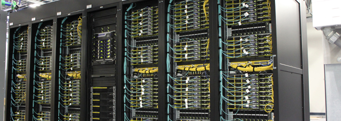
Linux Clusters
- From a hardware (and software) perspective, LC's GPU clusters are essentially the same as LC's other Linux clusters:
- Intel Xeon processor based
- InfiniBand interconnect
- Diskless, rack mounted "thin" nodes
- TOSS operating system/software stack
- Login nodes, compute nodes, gateway (I/O) and management nodes
- Compute nodes organized into partitions (pbatch, pdebug, pviz, etc.)
- Same compilers, debuggers and tools
- The only significant difference is that compute nodes (or a subset of compute nodes in the case of Max) include GPU hardware.
- Images below (click for larger image)

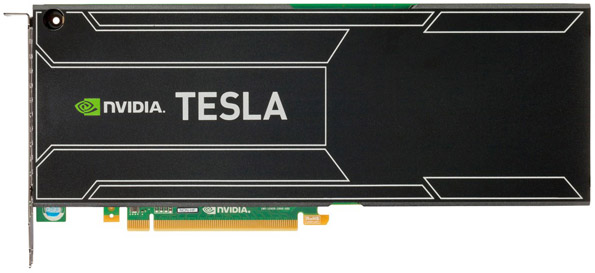
GPU Boards
- The NVIDIA Tesla GPUs are PCI Express Gen3 x16 @32 GB/s bidirectional peak (except for Max which is Gen2 @16 GB/s), dual-slot computing modules that plug into PCI-e x16 slots in the compute node.
- GPU boards vary in their memory, number of GPUs and type of GPUs. Some examples below (click for larger image).
Tesla K20 1
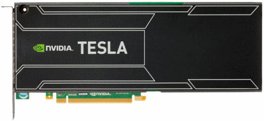

Tesla K40 2
Tesla K80 3


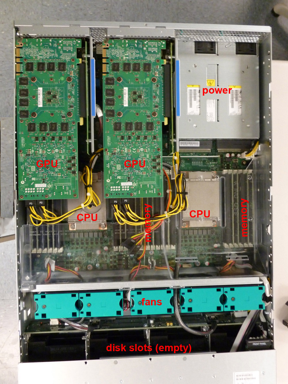
Compute Node 4
2 GPUs, 2 Sandy Bridge CPUs, no disk
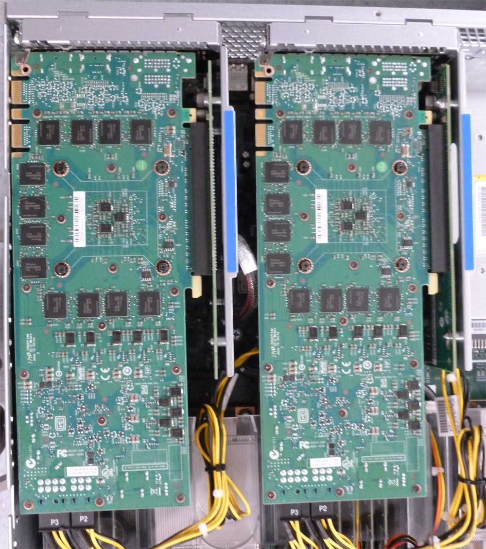
Tesla K40 GPU Boards 4
Close-up view; mounted bottom-side up
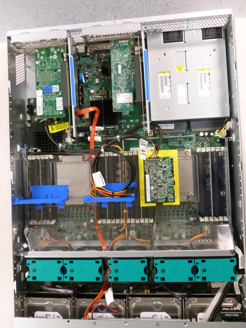
Non-compute Node 4
No GPUs, 2 Sandy Bridge CPUs, disk drives
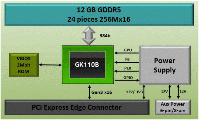
GPU Chip - Primary Components (Tesla K20, K40, K80)
-
Note For details on NVIDIA's Pascal GPU (used in LC's Pascal cluster), see the NVIDIA Tesla P100 Whitepaper.
The NVIDIA GPUs used in LC's Surface, RZHasgpu and Max clusters follow the basic design described below.
Streaming Multiprocessors (SMX): | These are the actual computational units. NVIDIA calls these SMX units. LC's clusters have 13, 14 or 15 SMX units per GPU. Each SMX unit has 192 CUDA cores. Discussed in more detail below.
L2 Cache: | Shared across the entire GPU. Amount of L2 cache varies by architecture. Primary point of data unification between the SMX units, servicing all load, store, and texture requests.
Memory Controllers: | Interfaces between the chip's L2 cache and the global on-board DRAM memory
PCI-e Interface: | PCI Express interface that connects the GPU to the host CPU(s). Primary function is to move data between the GPU and CPU memories.
Scheduling, Control, Graphics Hardware: | Specialized hardware that manages all other operations on the chip.
Photos / diagrams (click for larger image)

NVIDIA GK110 GPU Chip 6
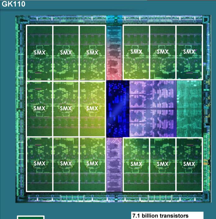
and Die 7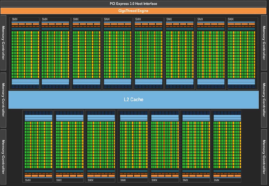
NVIDIA GK110-GK210 GPUs Block Diagram 8
Demonstrating primary GPU components
SMX Details (Tesla K20, K40, K80)
NoteFor details on NVIDIA's Pascal GPU (used in LC's Pascal cluster), see the NVIDIA Tesla P100 Whitepaper.
- The SMX unit is where the GPU's computational operations are performed.
- The number of SMX units per GPU chip varies, based on the type of GPU:
- Max: 14
- Surface: 15
- Rzhasgpu: 13
- SMX units have 192 single-precision CUDA cores
- Each CUDA core has one floating-point and one integer arithmetic unit; fully pipelined
- 64 double-precision (DP) units are used for double-precision math
- 32 special function units (SFU) are used for fast approximate transcendental operations
- Memory:
- GK110: 64 KB; divided between shared memory and L1 cache; configurable
- GK210: 128 KB; divided between shared memory and L1 cache; configurable
- 48 KB Read-Only Data Cache; both GK110 and GK210
- Register File:
- GK110: 65,536 x 32-bit
- GK210: 131,072 x 32-bit
- Other hardware:
- Instruction Cache
- Warp Scheduler
- Dispatch Units
- Texture Filtering Units (16)
- Load/Store Units (32)
- Interconnect Network
NVIDIA GK210 GPU SMX Block Diagram 8
Click for larger image
-
Additional Reading
- Surfing the web will turn up a wealth of information. A few links to NVIDIA Tesla hardware specs are provided below for convenience:
GPU Programming APIs: CUDA
Overview
- CUDA is both a parallel computing platform and an API for GPU programming.
- Created by NVIDIA (~2006) for use on its GPU hardware; does not currently run on non-NVIDIA hardware.
- CUDA originally stood for "Compute Unified Device Architecture", but this acronym is no longer used by NVIDIA.
- CUDA is accessible to developers through:
- CUDA accelerated libraries from NIVIDA and 3rd parties
- C/C++ compilers, such as nvcc from NVIDIA
- Fortran compilers, such as PGI's CUDA Fortran
- 3rd party wrappers for Python, Perl, Java, Ruby, Lua, MATLAB, IDL...
- Compiler directives, such as OpenACC
- NVIDIA's CUDA Toolkit is probably the most commonly used development environment:
- For C/C++ developers only
- Support for C++11
- C/C++ compiler (NVCC); based on the open source LLVM compiler infrastructure.
- GPU math libraries that provide single and double-precision C/C++ standard library math functions and intrinsics.
- GPU math libraries for FFT, BLAS, sparse matrix, dense and sparse direct solvers, random number generation, and more.
- Visual Profiler performance profiling tool (NVVP)
- CUDA-GDB debugger
- CUDA-MEMCHECK memory debugger
- Performance Primitives library (NPP) with GPU-accelerated image, video, and signal processing functions
- Graph Analytics library (nvGRAPH) providing parallel graph analytics
- Templated Parallel Algorithms & Data Structures (Thrust) library for GPU accelerated sort, scan, transform and reduction operations
- Nsight IDE plugin for Eclipse or Visual Studio
Basic Approach
The following steps describe a simple and typical scenario for developing CUDA code. Fully annotated vector addition example codes are provided, which you can pop open and view as you follow the steps below.
Follow Along:
- Identify which sections of code will be executed by the Host (CPU) and which sections by the Device (GPU).
- Device code is typically computationally intensive and able to be executed by many threads simultaneously in parallel.
- Host code is usually everything else
- Create kernels for the Device code:
- A kernel is a routine executed on the GPU as an array of threads in parallel
- Kernels are called from the Host
- Kernel syntax is similar to standard C/C++, but includes some CUDA extensions.
- All threads execute the same code
- Each thread has a unique ID
-
Example with CUDA extensions highlighted:
Standard C Routine CUDA C Kernel void vecAdd(double *a, double *b, double *c, int n) { for (int i = 0; i < n; ++i) c[i] = a[i] + b[i]; }__global__ void vecAdd(double *a, double *b, double *c, int n) { int i = blockIdx.x * blockDim.x + threadIdx.x; if (i < n) c[i] = a[i] + b[i]; } - Notes:
__global__ indicates a GPU kernel routine; must return void
blockIdx.x, blockDim.x, threadIdx.x are read-only built in variables used to compute each thread's unique ID as an index into the vectors
- Allocate space for data on the Host
- Use malloc as usual in your Host code
- Initialize data (typically)
-
Helpful convention: prepend Host variables with h_ to distinguish them from Device variables. Example:
h_a = (double*)malloc(bytes);
h_b = (double*)malloc(bytes);
h_c = (double*)malloc(bytes);
- Allocate space for data on the Device
- Done in Host code, but actually allocates Device memory
- Use CUDA routine such as cudaMalloc
-
Helpful convention: prepend Device variables with d_ to distinguish them from Host variables. Example:
cudaMalloc(&d_a, bytes);
cudaMalloc(&d_b, bytes);
cudaMalloc(&d_c, bytes);
- Copy data from the Host to the Device
- Done in Host code
- Use CUDA routine such as cudaMemcpy
-
Example:
cudaMemcpy(d_a, h_a, bytes, cudaMemcpyHostToDevice);
cudaMemcpy(d_b, h_b, bytes, cudaMemcpyHostToDevice);
- Set the number of threads to use; threads per block (blocksize) and blocks per grid (gridsize):
- Can have significant impact on performance; need to experiment
- Optimal settings vary by GPU, application, memory, etc.
- One tool (a spreadsheet) that can assist is the "CUDA Occupancy Calculator". Available from NVIDIA - just google it.
- Launch kernel from the Host to run on the Device
- Called from Host code but actually executes on Device
- Uses a special syntax clearly showing that a kernel is being called
- Need to specify the gridsize and blocksize from previous step
- Arguments depend upon your kernel
-
Example:
vecAdd<<<gridSize, blockSize>>>(d_a, d_b, d_c, n);
- Copy results back from the Device to the Host
- Done in Host code
- Use CUDA routine such as cudaMemcpy
-
Example:
cudaMemcpy(h_c, d_c, bytes, cudaMemcpyDeviceToHost);
- Deallocate Host and/or Device space if no longer needed:
- Done in Host code
-
Example:
 // Release host memory
free(h_a);
free(h_b);
free(h_c);
// Release device memory
cudaFree(d_a);
cudaFree(d_b);
cudaFree(d_c);
- Continue processing on Host, making additional data allocations, copies and kernel calls as needed.
Documentation and Further Reading
NVIDIA CUDA Zone: https://developer.nvidia.com/cuda-zone Recommended - one stop shop for everything CUDA.
- NVIDIA documentation installed on LC systems.
Complete and extensive set of manuals in pdf and html formats. Conveniently accessed online from all LC Linux clusters. See installation "doc" directories - for example: /opt/cudatoolkit/9.2/doc - "An Even Easier Introduction to CUDA": https://developer.nvidia.com/blog/even-easier-introduction-cuda
- CUDA Education & Training: https://developer.nvidia.com/cuda-education-training
- "CUDA Refresher: The CUDA Programming Model": https://developer.nvidia.com/blog/cuda-refresher-cuda-programming-model/
- "CUDA Programming on NVIDIA GPUs": http://people.maths.ox.ac.uk/~gilesm/cuda/
5-day hands-on CUDA programming course by Mike Giles from Oxford University. Lecture and exercise materials available online for free.
GPU Programming APIs: OpenMP
Overview
- OpenMP (Open Multi-Processing) is a parallel programming industry standard and API used to explicitly direct multi-threaded, shared memory parallelism.
- The most recent versions of the API also include support for GPUs/accelerators.
- Comprised of three primary API components:
- Compiler Directives
- Runtime Library Routines
- Environment Variables<
- Supports C, C++ and Fortran on most platforms and operating systems.
- Execution model:
- Main program running on Host begins as a serial thread (master thread) of execution.
- Regions of parallel execution are created as needed by the master thread
- Parallel regions are executed by a team of threads
- Work done by the team of threads in a parallel region can include loops or arbitrary blocks of code.
- Threads disband at the end of a parallel region and serial execution resumes until the next parallel region.
- Beginning with OpenMP4+, the programming model was expanded to include GPU/accelerators (Devices).
- Work is "offloaded" to a Device by using the appropriate compiler directives<
- Memory model:
- Without GPUs: OpenMP is a shared memory model. Threads can all access common, shared memory. They may also have their own private memory.
- With GPUs: Host and Device memories are separate and managed through directives.
- The OpenMP API is defined and directed by the OpenMP Architecture Review Board, comprised of a group of major computer hardware and software vendors, and major parallel computing user facilities.
Basic Approach
- Using OpenMP for non-GPU computing is covered in detail in LC's OpenMP Tutorial.
- Developing GPU OpenMP codes can be much simpler than CUDA, since it is mostly a matter of inserting compiler directives into existing code. For example, a simple, annotated vector addition example is shown below.
Follow Along:
- Identify which sections of code will be executed by the Host (CPU) and which sections by the Device (GPU).
- Device code is typically computationally intensive and able to be executed by many threads simultaneously in parallel.
- Host code is usually everything else
- Determine which data must be exchanged between the Host and Device
- Apply OpenMP directives to parallel regions and/or loops. In particular, use the OpenMP 4.5 "Device" directives.
- Apply OpenMP Device directives and/or directive clauses that define data transfer between Host and Device.
- In practice however, more work is usually needed in order to obtain improved/optimal performance. Other OpenMP directives, clauses and runtime library routines are used for such purposes as:
- Specifying the number of thread teams and distribution of work
- Collapsing loops
- Loop scheduling
Documentation and Further Reading
OpenMP.org official website: http://openmp.org
Recommended. Standard specifications, news, events, links to education resources, forums.
- Example codes for OpenMP 4.5. For GPU/accelerator related examples, see section 4 for Devices: http://www.openmp.org/wp-content/uploads/openmp-examples-4.5.0.pdf
- "Targeting GPUs with OpenMP 4.5 Device Directives": http://on-demand.gputechconf.com/gtc/2016/presentation/s6510-jeff-larkin-targeting-gpus-openmp.pdf
NVIDIA tutorial. Authors: James Beyer and Jeff Larkin, NVIDIA
GPU Programming APIs: OpenACC
Overview
- OpenACC (Open ACCelerators) is a parallel programming industry standard and API designed to simplify heterogeneous CPU + accelerator (e.g., GPU) programming.
- API consists primarily of compiler directives used to specify loops and regions of code to be offloaded from a host CPU to an attached accelerator, such as a GPU. Also includes 30+ runtime routines and a few environment variables.
- Designed for portability across operating systems, host CPUs, and a wide range of accelerators, including APUs, GPUs, and many-core coprocessors.
- C/C++ and Fortran interfaces
- Execution model:
- User application executes on Host
- Parallel regions and loops that can be executed on an attached Device are identified with compiler directives
- Multiple levels of parallelism are supported: gang, worker and vector:
- Gang: parallel regions/loops are executed on the Device by one or more gangs of workers; coarse grained; equivalent to a CUDA threadblock
- Worker: equivalent to a CUDA warp of threads; fine grained; may be vector enabled
- Vector: SIMD / vector operations that may occur within a worker; equivalent to CUDA threads in warp executing in SIMT lockstep
- User should not attempt to implement barrier synchronization, critical sections or locks across gang, worker or vector parallelism.
- Memory model: Host and Device memories are separate; all data movement between Host memory and Device memory must be performed by the Host through system calls that explicitly move data between the separate memories,
- Similar to OpenMP, which it is expected to merge with at some point.
- Developed by Cray, Nvidia, PGI and CAPS enterprise 9 (~2011). Currently includes over 20 member and supporter organizations.
Basic Approach
- Developing OpenACC codes can be much simpler than CUDA, since it is mostly a matter of inserting compiler directives into existing code. For example, a simple, annotated vector addition example is shown below.
Follow Along:
- Identify which sections of code will be executed by the Host (CPU) and which sections by the Device (GPU).
- Device code is typically computationally intensive and able to be executed by many threads simultaneously in parallel.
- Host code is usually everything else
- Determine which data must be exchanged between the Host and Device
- Apply OpenACC directives to parallel regions and/or loops.
- Apply OpenACC directives and/or directive clauses that define data transfer between Host and Device.
- In practice however, more work is usually needed in order to obtain improved/optimal performance. Other OpenACC directives, clauses and runtime library routines are used for such purposes as:
- Specifying the parallel scoping with gangs, workers, vectors
- Synchronizations
- Atomic operations
- Reductions
Documentation and Further Reading
OpenACC.org official website: http://www.openacc-standard.org/
Recommended. Standard specifications, news, events, links to education, software and application resources.
- OpenACC API 2.5 Reference Guide (local copy)
- NVIDIA OpenACC Tutorial (local copy)
GPU Programming APIs: OpenCL
Overview
OpenCL (Open Computing Language) is an open industry standard and framework for writing parallel programs that execute across heterogeneous platforms.
- Platforms may consist of central processing units (CPUs), graphics processing units (GPUs), digital signal processors (DSPs), field-programmable gate arrays (FPGAs) and other processors or hardware accelerators.
- The target of OpenCL is expert programmers wanting to write portable yet efficient code. Provides a low-level abstraction exposing details of the underlying hardware.
- Consists of a language (C/C++ based), an API, libraries and a runtime system.
- Execution model:
- Hardware consists of a Host connected to one or more OpenCL Devices.
- An OpenCL Device is divided into one or more compute units (CUs) which are further divided into one or more processing elements (PEs). Computations on a device occur within the processing elements.
- An OpenCL application is implemented as both Host code and Device kernel code. These are two distinct units of execution.
- Host code runs on a host processor according to the models native to the host platform.
- Device kernel code is where the computational work is done. It is called as a command from the Host code, and executes on an OpenCL Device.
- The Host manages the execution context/environment of kernels.
- The Host also interacts with kernels through a command-queue provided by the API. Permits specification of memory transactions and synchronization points.
- Work executed on a Device is decomposed into work-items, work-groups and work-subgroups. For details, see the API specs.
- Memory model:
- Memory in OpenCL is divided into two parts: Host memory and Device memory.
- Device memory is further divided into 4 memory regions: Global, Constant, Local and Private memory address space.
- Beyond this, the OpenCL memory model is complex and requires understanding the API specs in detail.
- OpenCL is an open standard maintained by the non-profit technology consortium Khronos Group.
- OpenCL is not discussed further in this document, as it is not commonly used or supported at LC.
Documentation and Further Reading
Khronos Group website: https://www.khronos.org/opencl Recommended. Standard specifications, software, resources, documentation, forums
Compiling
Compiling: CUDA
The following instructions apply to LC's TOSS 3 Linux GPU clusters:
C/C++
- NVIDIA CUDA software is directly accessible under /opt/cudatoolkit/.
-
Alternately, you may load an NVIDIA CUDA Toolkit module:
module load opt (load the opt module first) module avail cuda (display available cuda modules) module load cudatoolkit/9.2 (load a recent CUDA toolkit module) - Source files containing CUDA code should be named with a .cu suffix. For example: myprog.cu
-
Use NVIDIA's C/C++ nvcc compiler to compile your source files. Mixing .cu with .c or .cc is fine. For example:
nvcc sub1.cu sub2.c myprog.cu -o myprog
- Note: nvcc is actually a compiler driver and depends upon gcc as the native C/C++ compiler. Details can be found in the nvcc documentation.
Fortran
- Source files containing CUDA code should be named with a .cuf suffix. For example: myprog.cuf
-
Load a recent PGI compiler package:
module avail pgi (display available PGI compiler packages) module load pgi/18.5 (load a recent version) -
Use the PGI pgfortran, pgf90 or pgf95 compiler command to compile your source files. Mixing .cuf with .f or .f90 is fine. For example:
pgfortran sub1.cuf sub2.f myprog.f -o myprog
- Optional: if you want to use tools from the NVIDIA CUDA Toolkit, you'll need to load an NVIDIA cudatoolkit module, as shown in the C/C++ example above.
Getting Help
- C/C++
- Use the nvcc --help command
- See the NVIDIA documentation installed in the /doc subdirectory /opt/cudatoolkit/version/.
- Consult NVIDIA's documentation online at nvidia.com
- Fortran:
- pgfortran, pgf90, pgf95 man page - see the -Mcuda section
Compiling: OpenMP
Current Situation for LC's Linux Commodity Clusters
- The OpenMP 4.0 and 4.5 APIs provide constructs for GPU "Device" computing. OpenMP 4.5 in particular, provides support for offloading computations to GPUs.
- Support for these constructs varies between compilers.
- Support for OpenMP 4.5 offloading for NVIDIA GPU hardware is not expected from Intel or PGI anytime soon.
- GCC supports OpenMP 4.5 offloading in version 6.1, but only for Intel Knights Landing and AMD HSAIL. Support for NVDIA GPUs may come later.
- The Clang open-source C/C++ compiler OpenMP 4.5 offloading support for NVIDIA GPUs is under development and is expected to become available in a future version.
- The OpenMP website maintains of list of compilers and OpenMP support at: https://www.openmp.org/resources/openmp-compilers-tools/.
- In summary: there's not much available yet...
Compiling: OpenACC
Load Required Modules
-
Load a PGI compiler package:
module avail pgi (display available PGI compiler packages) module load pgi/18.5 (load a recent version) -
Optional: load a recent NVIDIA cudatoolkit module. This is only needed if you plan on using NVIDIA profiling/debugging tools, such as nvprof or nvvp:
module load opt (load the opt module first) module avail cuda (display available cuda modules) module load cudatoolkit/9.2 (load a recent CUDA toolkit module) - Alternately, the NVIDIA CUDA software is directly accessible under /opt/cudatoolkit/.
Compile Using a PGI Compiler Command
-
Use the appropriate PGI compiler command, depending upon the source code type.
Language Compiler Command Flags Notes C pgcc -acc
-Minfo
-Minfo=acc- Same flags apply to all compiler commands.
- -acc flag is required to turn on OpenACC source code directives.
- -Minfo reports compiler optimizations. -Minfo=acc reports only optimizations related to parallelization and GPU code.
- Other compiler flags may be used as desired.
- pgf77 is not available for OpenACC
C++ pgCC Fortran pgfortran
pgf90 -
Example:
% pgcc -acc -Minfo=acc -fast matmult.c
main:
     24, Generating copyin(a[:][:],b[:][:])
         Generating copy(c[:][:])
     25, Loop is parallelizable
     26, Loop is parallelizable
     27, Complex loop carried dependence of c prevents parallelization
         Loop carried dependence of c prevents parallelization
         Loop carried backward dependence of c prevents vectorization
         Inner sequential loop scheduled on accelerator
         Accelerator kernel generated
         Generating Tesla code
         25, #pragma acc loop gang /* blockIdx.y */
         26, #pragma acc loop gang, vector(128) /* blockIdx.x threadIdx.x */
Misc. Tips & Tools
The following information applies to LC's Linux GPU clusters surface, max and rzhasgpu.
Running Jobs
- Make sure that you are actually on a compute node with a GPU:
- Login nodes do NOT have GPUs
- max: be sure to specify the pgpu partition, as these are the only nodes with GPUs.
- surface: all compute nodes in pbatch are NVIDIA K40m GPUs. Compute nodes in GPGPU are NVIDIA M60 GPUs.
- rzhasgpu: all compute nodes (pdebug, pbatch, etc.) have GPUs.
- At runtime, on a GPU node, you may need to load the same modules/dotkits that you used when you built your executable. Depends on the situation and what you want to do.
- Visualization jobs have priority on surface and max GPU nodes. Users who are not running visualization work, should run in standby mode:
- Include #MSUB -l qos=standby in your batch script
- Or, submit your job with msub -l qos=standby
- Standy jobs can be preempted (terminated) if a non-standby job requires their nodes.
- Non-visualization jobs not using standby may be terminated
GPU Hardware Info
- deviceQuery: command to display a variety of GPU hardware information. Must be executed on a node that actually has GPUs.
-
You may need to build this yourself if LC hasn't already, or if it's not in your path. Typically found under:
/opt/cudatoolkit/version/samples/1_Utilities/deviceQuery
Example output below:
% deviceQuery ./deviceQuery Starting... CUDA Device Query (Runtime API) version (CUDART static linking) Detected 2 CUDA Capable device(s) Device 0: "Tesla P100-PCIE-16GB" CUDA Driver Version / Runtime Version 9.2 / 9.1 CUDA Capability Major/Minor version number: 6.0 Total amount of global memory: 16281 MBytes (17071734784 bytes) (56) Multiprocessors, ( 64) CUDA Cores/MP: 3584 CUDA Cores GPU Max Clock rate: 1329 MHz (1.33 GHz) Memory Clock rate: 715 Mhz Memory Bus Width: 4096-bit L2 Cache Size: 4194304 bytes Maximum Texture Dimension Size (x,y,z) 1D=(131072), 2D=(131072, 65536), 3D=(16384, 16384, 16384) Maximum Layered 1D Texture Size, (num) layers 1D=(32768), 2048 layers Maximum Layered 2D Texture Size, (num) layers 2D=(32768, 32768), 2048 layers Total amount of constant memory: 65536 bytes Total amount of shared memory per block: 49152 bytes Total number of registers available per block: 65536 Warp size: 32 Maximum number of threads per multiprocessor: 2048 Maximum number of threads per block: 1024 Max dimension size of a thread block (x,y,z): (1024, 1024, 64) Max dimension size of a grid size (x,y,z): (2147483647, 65535, 65535) Maximum memory pitch: 2147483647 bytes Texture alignment: 512 bytes Concurrent copy and kernel execution: Yes with 2 copy engine(s) Run time limit on kernels: No Integrated GPU sharing Host Memory: No Support host page-locked memory mapping: Yes Alignment requirement for Surfaces: Yes Device has ECC support: Enabled Device supports Unified Addressing (UVA): Yes Supports Cooperative Kernel Launch: Yes Supports MultiDevice Co-op Kernel Launch: Yes Device PCI Domain ID / Bus ID / location ID: 0 / 4 / 0 Compute Mode: Exclusive Process (many threads in one process is able to use ::cudaSetDevice() with this device) ... -
nvidia-smi: NVIDIA System Management Interface utility. Provides monitoring and management capabilities for NVIDIA GPUs. Example below - see man page, or use with -h flag for details.
% nvidia-smi
Thu Mar 16 10:10:53 2017
+-----------------------------------------------------------------------------+
| NVIDIA-SMI 367.48                 Driver Version: 367.48                    |
|-------------------------------+----------------------+----------------------+
| GPU  Name        Persistence-M| Bus-Id        Disp.A | Volatile Uncorr. ECC |
| Fan  Temp  Perf  Pwr:Usage/Cap|         Memory-Usage | GPU-Util  Compute M. |
|===============================+======================+======================|
|   0  Tesla K40m          On   | 0000:08:00.0     Off |                    0 |
| N/A   22C    P8    19W / 235W |      0MiB / 11439MiB |      0%   E. Process |
+-------------------------------+----------------------+----------------------+
|   1  Tesla K40m          On   | 0000:82:00.0     Off |                    0 |
| N/A   20C    P8    19W / 235W |      0MiB / 11439MiB |      0%   E. Process |
+-------------------------------+----------------------+----------------------+

+-----------------------------------------------------------------------------+
| Processes:                                                       GPU Memory |
|  GPU       PID  Type  Process name                               Usage      |
|=============================================================================|
|  No running processes found                                                 |
+-----------------------------------------------------------------------------+
Debuggers, Tools
-
NVIDIA's nvprof is a simple to use, text based profiler for GPU codes. To use it, make sure your cudatoolkit module is loaded, and then call it with your executable. For example:
% module list
Currently Loaded Modulefiles:
  1) java/1.8.0        2) cudatoolkit/9.2

% nvprof a.out
==60828== NVPROF is profiling process 60828, command: a.out
final result: 1.000000
==60828== Profiling application: a.out
==60828== Profiling result:
Time(%)      Time     Calls       Avg       Min       Max  Name
 64.14%  217.82us         2  108.91us  108.42us  109.41us  [CUDA memcpy HtoD]
 31.86%  108.19us         1  108.19us  108.19us  108.19us  [CUDA memcpy DtoH]
  4.00%  13.568us         1  13.568us  13.568us  13.568us  vecAdd(double*, double*, double*, int)

==60828== API calls:
Time(%)      Time     Calls       Avg       Min       Max  Name
 98.88%  536.81ms         3  178.94ms  219.99us  536.37ms  cudaMalloc
  0.63%  3.3933ms       332  10.220us     101ns  474.13us  cuDeviceGetAttribute
  0.18%  955.34us         3  318.45us  86.272us  691.17us  cudaMemcpy
  0.17%  946.59us         4  236.65us  218.84us  259.55us  cuDeviceTotalMem
  0.09%  504.55us         3  168.18us  154.05us  192.83us  cudaFree
  0.05%  244.76us         4  61.189us  55.944us  72.734us  cuDeviceGetName
  0.00%  26.266us         1  26.266us  26.266us  26.266us  cudaLaunch
  0.00%  2.8030us         4     700ns     180ns  2.0840us  cudaSetupArgument
  0.00%  2.0060us         2  1.0030us     189ns  1.8170us  cuDeviceGetCount
  0.00%  1.0600us         8     132ns      94ns     239ns  cuDeviceGet
  0.00%     969ns         1     969ns     969ns     969ns  cudaConfigureCall
- NVIDIA's Visual Profiler, nvvp is a very full featured, graphical profiler and performance analysis tool. It can provide very detailed information about how your code is using the GPU.
- To start it up, make sure your cudatoolkit and java modules are loaded, and then invoke it with your executable - as for nvprof above.
- See NVIDIA's documentation for more information.
- Screen shot below - click for larger image
- NVIDIA Nsight provides a complete development platform for heterogeneous computing, that includes debugging and profiling tools. See NVIDIA's documentation for details.
- Debugging: several choices are available. See the respective documentation for details.
- NVIDIA cuda-debug
- NVIDIA cuda-memcheck
- TotalView
- Allinea DDT
NOTE: This completes the tutorial.
Pease complete the online evaluation form - unless you are doing the exercise, in which case please complete it at the end of the exercise.
Where would you like to go now?
References and More Information
- Original Author: Blaise Barney; Contact: hpc-tutorials@llnl.gov, Livermore Computing.
- Hardware/Vendor Information:
- AMD: amd.com
- Intel: intel.com
- Mellanox: mellanox.com
- QLogic: qlogic.com
- Voltaire: voltaire.com
- SLURM Documentation: http://slurm.schedmd.com
- Linux Project Report: 2002 Linux Project Report
- Credits/Sources
- 1 NVIDIA: Tesla K20 GPU Accelerator Board Specification. BD-06455-001_v07, July 2013
- 2 NVIDIA: Tesla K40 GPU Accelerator Board Specification. BD-06902-001_v05, November 2013
- 3 NVIDIA: Tesla K80 GPU Accelerator Board Specification. BD-07317-001_v05, January 2015
- 4 Blaise Barney, LLNL. Livermore Computing's Surface cluster. April 2016
- 5 Adam Bertsch, LLNL. Livermore Computing's Surface cluster.
- 6 wikipedia.com
- 7 NVIDIA Whitepaper: NVIDIA's Next Generation CUDA Compute Architecture: Kepler GK110/210 V1.0. 2014. Annotations by Blaise Barney, LLNL
- 8 NVIDIA Whitepaper: NVIDIA's Next Generation CUDA Compute Architecture: Kepler GK110/210 V1.0. 2014.