
NOTE This tutorial is fully deprecated as of early 2026.
Table of Contents
- Abstract
- Quickstart Guide
- Sierra Overview
- Sierra Hardware
- Accounts, Allocations and Banks
- Accessing LC's Sierra Machines
- Software and Development Environment
- Compilers on Sierra
- MPI
- OpenMP
- System Configuration and Status Information
- Running Jobs on Sierra Systems
- Summary of Job-Related Commands
- Batch Scripts and #BSUB / bsub
- Interactive Jobs: bsub and lalloc commands
- Launching Jobs: the lrun Command
- Launching Jobs: the jsrun Command and Resource Sets
- Job Dependencies
- Monitoring Jobs: lsfjobs, bquery, bpeek, bhist commands
- Suspending / Resuming Jobs: bstop, bresume commands
- Modifying Jobs: bmod command
- Signaling / Killing Jobs: bkill command
- CUDA-aware MPI
- Process, Thread and GPU Binding: js_task_info
- Node Diagnostics: check_sierra_nodes
- Burst Buffer Usage
- Banks, Job Usage and Job History Information
- LSF - Additional Information
- Math Libraries
- Debugging
- Performance Analysis Tools
- Tutorial Evaluation
- References & Documentation
- Appendix A: Quickstart Guide
Abstract
This tutorial is intended for users of Livermore Computing's Sierra systems. It begins by providing a brief background on CORAL, leading to the CORAL EA and Sierra systems at LLNL. The CORAL EA and Sierra hybrid hardware architectures are discussed, including details on IBM POWER8 and POWER9 nodes, NVIDIA Pascal and Volta GPUs, Mellanox network hardware, NVLink and NVMe SSD hardware.
Information about user accounts and accessing these systems follows. User environment topics common to all LC systems are reviewed. These are followed by more in-depth usage information on compilers, MPI and OpenMP. The topic of running jobs is covered in detail in several sections, including obtaining system status and configuration information, creating and submitting LSF batch scripts, interactive jobs, monitoring jobs and interacting with jobs using LSF commands.
A summary of available math libraries is presented, as is a summary on parallel I/O. The tutorial concludes with discussions on available debuggers and performance analysis tools.
A Quickstart Guide is included as an appendix to the tutorial, but it is linked at the top of the tutorial table of contents for visibility.
Level/Prerequisites: Intended for those who are new to developing parallel programs in the Sierra environment. A basic understanding of parallel programming in C or Fortran is required. Familiarity with MPI and OpenMP is desirable. The material covered by EC3501 - Introduction to Livermore Computing Resources would also be useful.
Sierra Overview
CORAL:

- C O R A L = Collaboration of Oak Ridge, Argonne, and Livermore
- A first-of-its-kind U.S. Department of Energy (DOE) collaboration between the NNSA's ASC Program and the Office of Science's Advanced Scientific Computing Research program (ASCR).
- CORAL is the next major phase in the DOE's scientific computing roadmap and path to exascale computing.
- Will culminate in three ultra-high performance supercomputers at Lawrence Livermore, Oak Ridge, and Argonne national laboratories.
- Will be used for the most demanding scientific and national security simulation and modeling applications, and will enable continued U.S. leadership in computing.
- The three CORAL systems are:
- LLNL and ORNL systems were delivered in the 2017-18 timeframe. The Argonne system's planned delivery (revised) is in 2021.
- DOE / NNSA CORAL Fact Sheet (Dec 17, 2014)
- Announcements/Press:
CORAL Early Access (EA) Systems

- In preparation for the final delivery Sierra systems, LLNL implemented three "early access" systems, one on each network:
- ray - OCF-CZ
- rzmanta - OCF-RZ
- shark - SCF
- Primary purpose was to provide platforms where Tri-lab users could begin porting and preparing for the hardware and software that would be delivered with the final Sierra systems.
- Similar to the final delivery Sierra systems but use the previous generation IBM Power processors and NVIDIA GPUs.
- IBM Power Systems S822LC Server:
- Hybrid architecture using IBM POWER8+ processors and NVIDIA Pascal GPUs.
- IBM POWER8+ processors:
- 2 per node (dual-socket)
- 10 cores/socket; 20 cores per node
- 8 SMT threads per core; 160 SMT threads per node
- Clock: due to adaptive power management options, the clock speed can vary depending upon the system load. At LC speeds can vary from approximately 2 GHz - 4 GHz.
- NVIDIA GPUs:
- 4 NVIDIA Tesla P100 (Pascal) GPUs per compute node (not on login/service nodes)
- 3584 CUDA cores per GPU; 14,336 per node
- Memory:
- 256 GB DDR4 per node
- 16 GB HBM2 (High Bandwidth Memory 2) per GPU; 732 GB/s peak bandwidth
- NVLINK 1.0:
- Interconnect for GPU-GPU and CPU-GPU shared memory
- 4 links per GPU/CPU with 160 GB/s total bandwidth (bidirectional)
- NVRAM:
- 1.6 TB NVMe PCIe SSD per compute node (CZ ray system only)
- Network:
- Mellanox 100 Gb/s Enhanced Data Rate (EDR) InfiniBand
- One dual-port 100 Gb/s EDR Mellanox adapter per node
- Parallel File System: IBM Spectrum Scale (GPFS)
- ray: 1.3 PB
- rzmanta: 431 TB
- shark: 431 TB
- Batch System: IBM Spectrum LSF
- System Details:
| CORAL Early Access (EA) Systems | |||||||||||
|---|---|---|---|---|---|---|---|---|---|---|---|
| Cluster | OCF SCF |
Architecture | Clock Speed (GHz) | Nodes GPUs |
Cores /Node /GPU |
Cores Total | Memory/ Node (GB) |
Memory Total (GB) |
TFLOPS Peak |
Switch | ASC M&IC |
| ray | OCF | IBM Power8 NVIDIA Tesla P100 (PASCAL) |
2.0-4.0 1481 MHz |
62 54*4 |
20 3484 |
1,240 752,544 |
256 16*4 |
15,872 3,456 |
39.7 1,144.8 |
IB EDR | ASC/M&IC |
| rzmanta | OCF | IBM Power8 NVIDIA Tesla P100 (PASCAL) |
2.0-4.0 1481 MHz |
44 36*4 |
20 3484 |
880 501,696 |
256 16*4 |
11,264 2,304 |
28.2 763.2 |
IB EDR | ASC |
| shark | SCF | IBM Power8 NVIDIA Tesla P100 (PASCAL) |
2.0-4.0 1481 MHz |
44 36*4 |
20 3484 |
880 501,696 |
256 16*4 |
11,264 2,304 |
28.2 763.2 |
IB EDR | ASC |
- Additional information:
- User Guide: https://lc.llnl.gov/confluence/display/CORALEA/CORAL+EA+Systems (LC internal wiki)
- ray configuration: https://hpc.llnl.gov/hardware/platforms/Ray
- rzmanta configuration: https://hpc.llnl.gov/hardware/platforms/RZManta
- shark configuration: https://hpc.llnl.gov/hardware/platforms/Shark
Sierra Systems

- Sierra is a classified, 125 petaflop, IBM Power Systems AC922 hybrid architecture system comprised of IBM POWER9 nodes with NVIDIA Volta GPUs. Sierra is a Tri-lab resource sited at Lawrence Livermore National Laboratory.
- Unclassified Sierra systems are similar, but smaller, and include:
- lassen - a 22.5 petaflop system located on LC's CZ zone.
- rzansel - a 1.5 petaflop system is located on LC's RZ zone.
- IBM Power Systems AC922 Server:
- Hybrid architecture using IBM POWER9 processors and NVIDIA Volta GPUs.
- IBM POWER9 processors (compute nodes):
- 2 per node (dual-socket)
- 22 cores/socket; 44 cores per node
- 4 SMT threads per core; 176 SMT threads per node
- Clock: due to adaptive power management options, the clock speed can vary depending upon the system load. At LC speeds can vary from approximately 2.3 - 3.8 GHz. LC can also set the clock to a specific speed regardless of workload.
- NVIDIA GPUs:
- 4 NVIDIA Tesla V100 (Volta) GPUs per compute, login, launch node
- 5120 CUDA cores per GPU; 20,480 per node
- Memory:
- 256 GB DDR4 per compute node; 170 GB/s peak bandwidth (per socket)
- 16 GB HBM2 (High Bandwidth Memory 2) per GPU; 900 GB/s peak bandwidth
- NVLINK 2.0:
- Interconnect for GPU-GPU and CPU-GPU shared memory
- 6 links per GPU/CPU with 300 GB/s total bandwidth (bidirectional)
- NVRAM:
- 1.6 TB NVMe PCIe SSD per compute node
- Network:
- Mellanox 100 Gb/s Enhanced Data Rate (EDR) InfiniBand
- One dual-port 100 Gb/s EDR Mellanox adapter per node
- Parallel File System: IBM Spectrum Scale (GPFS)
- Batch System: IBM Spectrum LSF
- Water (warm) cooled compute nodes
- System Details:
| Sierra Systems (compute nodes) | |||||||||||
|---|---|---|---|---|---|---|---|---|---|---|---|
| Cluster | OCF SCF |
Architecture | Clock Speed (GHz) | Nodes GPUs |
Cores /Node /GPU |
Cores Total | Memory/ Node (GB) |
Memory Total (GB) |
TFLOPS Peak |
Switch | ASC M&IC |
| sierra | SCF | IBM Power9 NVIDIA TeslaV100 (Volta) |
2.3-3.8 1530 MHz |
4320 4320*4 |
44 5120 |
190,080 88,473,600 |
256 16*4 |
1,105,920 276,480 |
125,000 | IB EDR | ASC |
| lassen | OCF | IBM Power9 NVIDIA TeslaV100 (Volta) |
2.3-3.8 1530 MHz |
774 774*4 |
44 5120 |
34,056 15,851,520 |
256 16*4 |
198,144 49,536 |
22,508 | IB EDR | ASC/M&IC |
| rzansel | OCF | IBM Power9 NVIDIA TeslaV100 (Volta) |
2.3-3.8 1530 MHz |
54 54*4 |
44 5120 |
2376 1,105,920 |
256 16*4 |
13,824 3,456 |
1,570 | IB EDR | ASC |
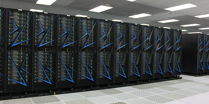
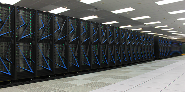
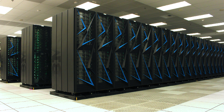
Photos

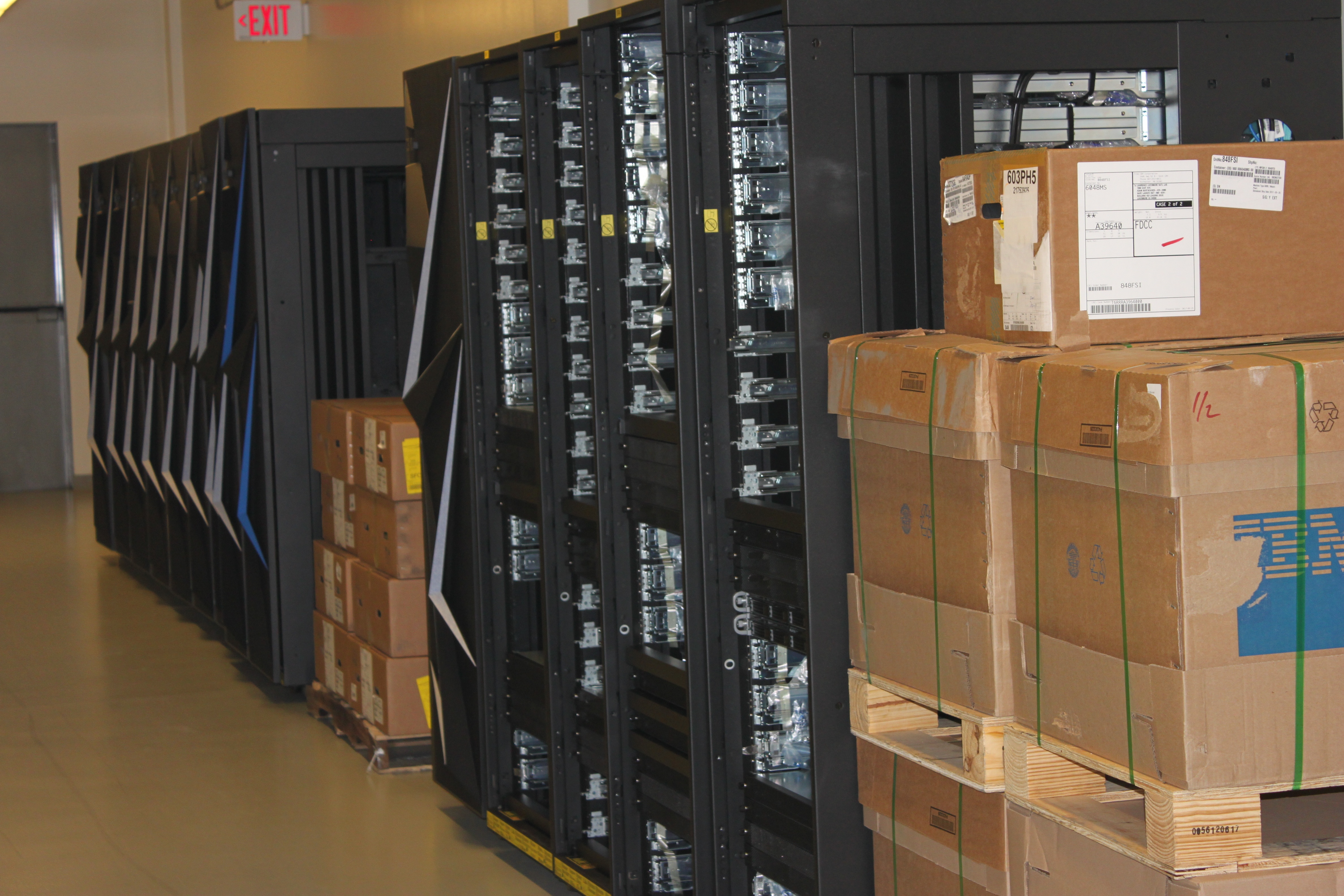
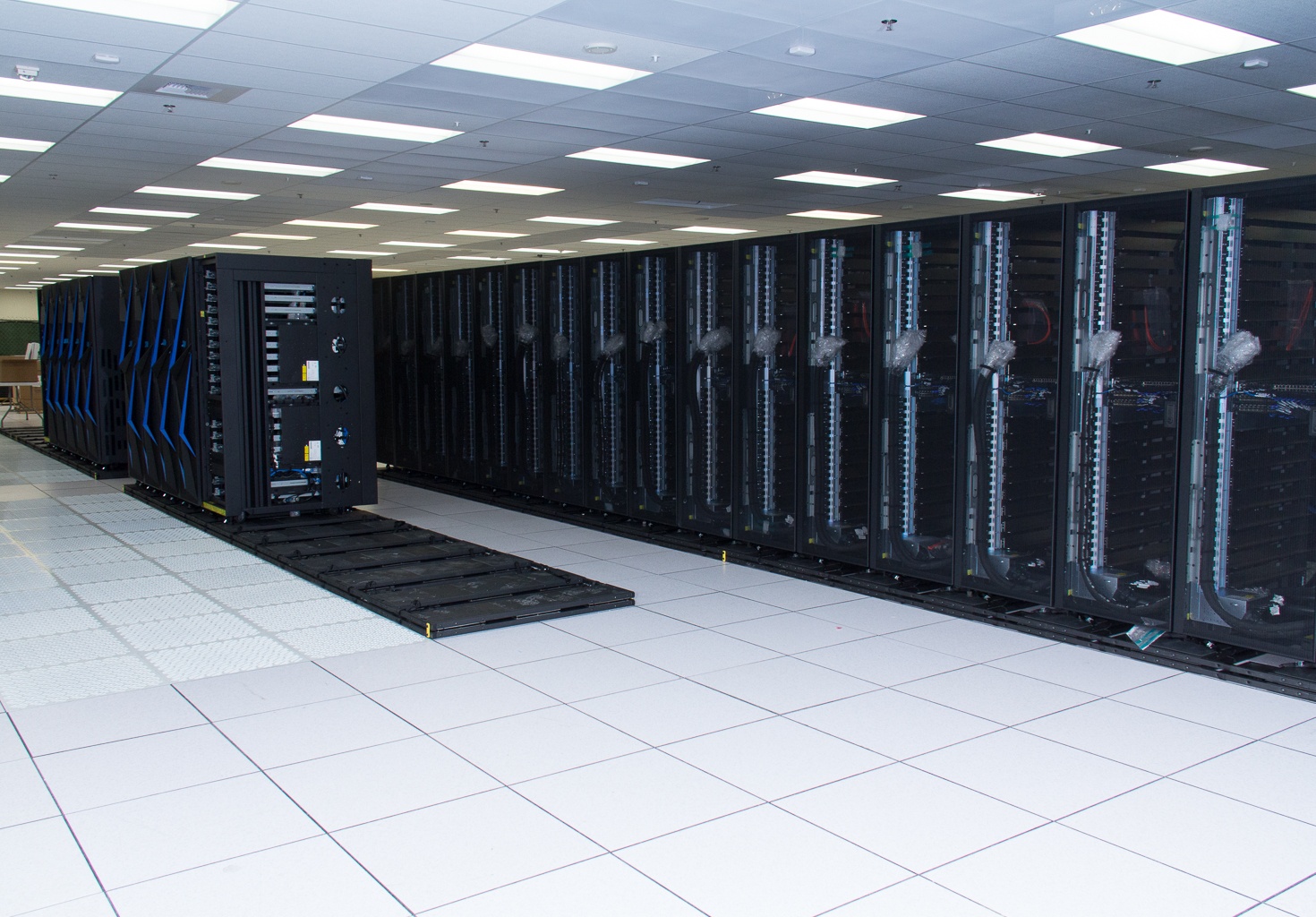
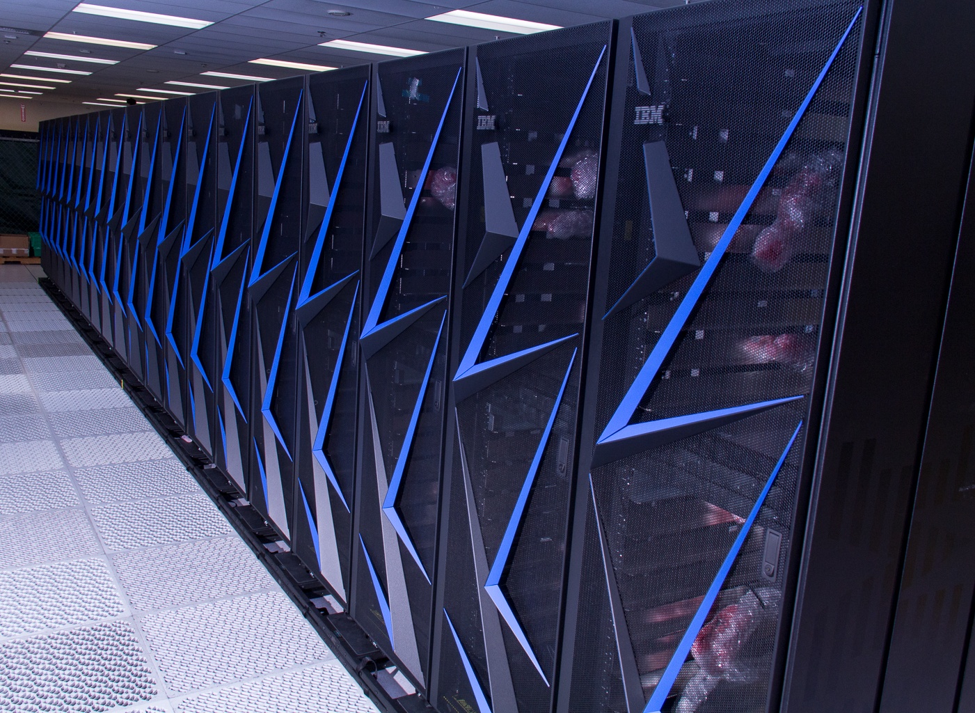
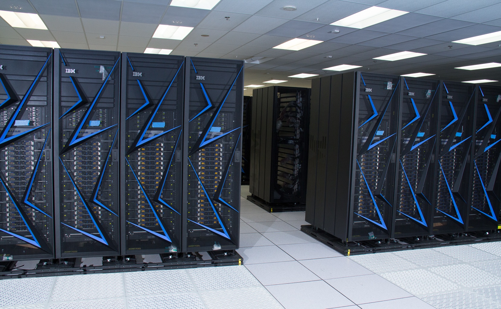
Hardware
Sierra Systems General Configuration
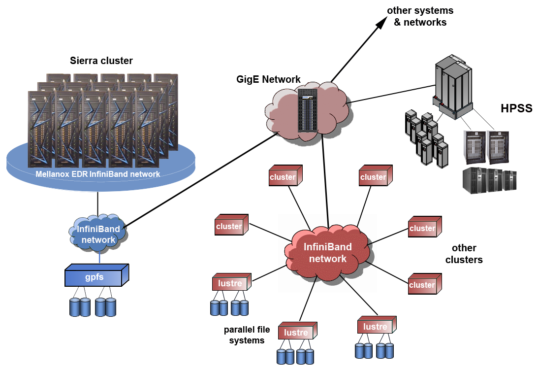
System Components
- The basic components of a Sierra system are the same as other LC systems. They include:
- Frames / Racks
- Nodes
- File Systems
- Networks
- HPSS Archival Storage
Frames / Racks
- Frames are the physical cabinets that hold most of a cluster's components:
- Nodes of various types
- Switch components
- Other network and cluster management components
- Parallel file system disk resources (usually in separate racks)
- Power and console management - frames include hardware and software that allow system administrators to perform most tasks remotely.
Nodes
- Sierra systems consist of several different node types:
- Compute nodes
- Login / Launch nodes
- I/O nodes
- Service / management nodes
- Compute Nodes:
- Comprise the heart of a system. This is where parallel user jobs run.
- Dual-socket IBM POWER9 (AC922) nodes
- 4 NVIDIA Tesla V100 (Volta) GPUs per node
- Login / Launch Nodes:
- When you connect to Sierra, you are placed on a login node. This is where users perform interactive, non-production work: edit files, launch GUIs, submit jobs and interact with the batch system.
- Launch nodes are similar to login nodes, but are dedicated to managing user jobs, which in turn launch parallel jobs on compute nodes using jsrun (discussed later).
- Login / launch nodes are shared by multiple users and should not be used themselves to run parallel jobs.
- IBM Power9 with 4 NVIDIA Volta GPUs (same as compute nodes)
- I/O Nodes:
- Dedicated file servers for IBM Spectrum Scale parallel file systems
- Not directly accessible to users
- IBM Power9, dual-socket; no GPUs
- Service / Management Nodes:
- Reserved for system related functions and services
- Not directly accessible to users
- IBM Power9, dual-socket; no GPUs
Networks
- Sierra systems have a Mellanox 100 Gb/s Enhanced Data Rate (EDR) InfiniBand network:
- Internal, inter-node network for MPI communications and I/O traffic between compute nodes and I/O nodes.
- See the Mellanox EDR InfiniBand Network section for details.
- InfiniBand networks connect other clusters and parallel file servers.
- A GigE network connects InfiniBand networks, HPSS and external networks and systems.
File Systems
- Parallel file systems: Sierra systems use IBM Spectrum Scale. Other clusters use Lustre.
- Other file systems (not shown) such as NFS (home directories, temp) and infrastructure services
Archival HPSS Storage
- Details and usage information available at: https://hpc.llnl.gov/training/tutorials/livermore-computing-resources-and-environment#Archival.
IBM POWER8 Architecture
Used by LLNL's Early Access systems ray, rzmanta, shark
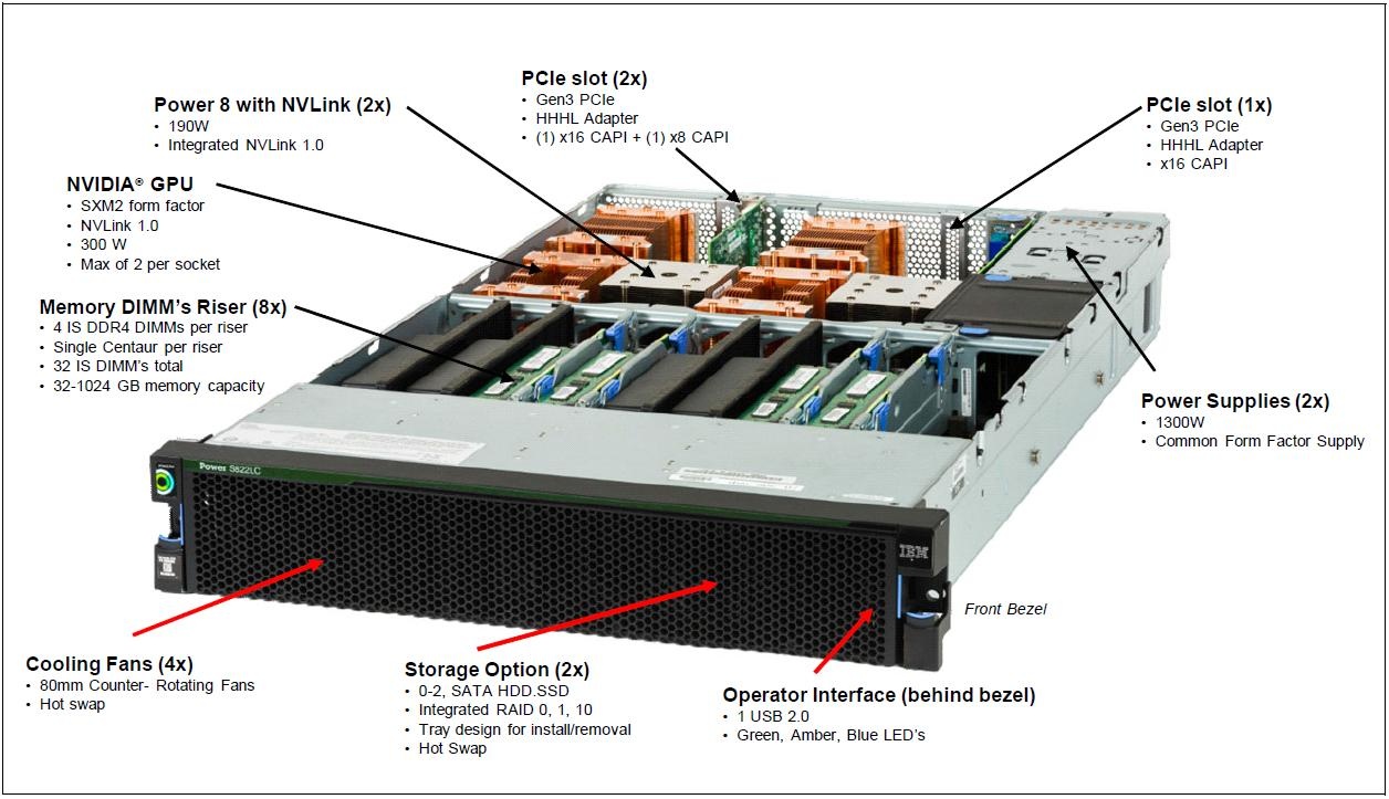
IBM POWER8 SL822LC Node Key Features
- 2 IBM "POWER8+" processors (dual-socket)
- Up to 4 NVIDIA Tesla P100 (Pascal) GPUs
- NVLink GPU-CPU and GPU-GPU interconnect technology
- Memory:
- Up to 1024 GB DDR4 memory per node
- LC's Early Access systems compute nodes have 256 GB memory
- Each processor connects to 4 memory riser cards with 4 DIMMs;
- Processor-to-memory peak bandwidth of 115 GB/s bandwidth per processor, 230 GB/s memory bandwidth per node
- L4 cache: up to 64 MB per processor, in 16 MB banks of memory buffers
- Storage: 2 disk bays for 2 hard disk drives (HDD) or 2 solid state drives (SSD). Optional NVMe SSD support in PCIe slots.
- Coherent Accelerator Processor Interface (CAPI), which allows accelerators plugged into a PCIe slot to access the processor bus by using a low latency, high-speed protocol interface.
- 5 integrated PCIe Gen 3 slots:
- 1 PCIe x8 G3 LP slot, CAPI enabled
- 1 PCIe x16 G3, CAPI enabled
- 1 PCIe x8 G3
- 2 PCIe x16 G3, CAPI enabled that support GPU or PCIe adapters
- Adaptive power management
- I/O ports: 2x USB 3.0; 2x 1 GB Ethernet; VGA
- 2 hotswap, redundant power supplies (no power redundancy with GPU(s) installed)
- 19-inch rackmount hardware (2U)
- LLNL's Early Access POWER8 nodes:
- Compute nodes are model 8335-GTB and login nodes are model 8335-GCA. The primary difference is that compute nodes include 4 NVIDIA Pascal GPUs and Power8 processors with NVLink technology.
- Power8 processors use 10 cores
- Memory: 256 GB per node
- The CZ Early Access cluster "Ray" also has 1.6 TB NVMe PCIe SSD (attached solid state storage).
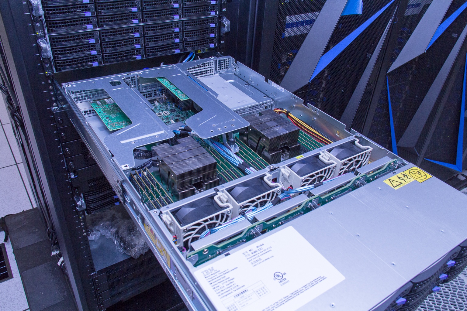
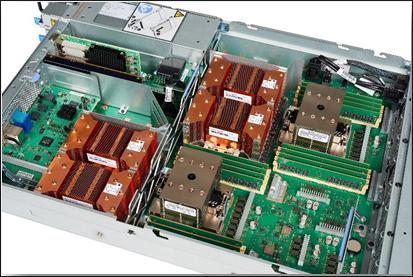
- Images
- A POWER8 compute node and its primary components are shown below. Relevant individual components are discussed in more detail in sections below.
- Click for a larger image. (Source: "IBM Power Systems S822LC for High Performance Computing Technical Overview and Introduction". IBM Redpaper publication REDP-5405-00 by Alexandre Bicas Caldeira, Volker Haug, Scott Vetter. September, 2016)

POWER8 Processor Key Characteristics
- IBM 22 nm Silicon-On-Insulator (SOI) technology; 4.2 billion transistors
- Up to 12 cores (LLNL's Early Access processors have 10 cores)
- L1 data cache: 64 KB per core, 8-way, private
- L1 instruction cache: 32 KB per core, 8-way, private
- L2 cache: 512 KB per core, 8-way, private
- L3 cache: 96 MB (12 core version), 8-way, shared as 8 MB banks per core
- Hardware transactional memory
- Clock: due to adaptive power management options, the clock speed can vary depending upon the system load. At LLNL speeds can vary from approximately 2 GHz - 4 GHz.
- Images:
- Images of the POWER8 processor chip (12 core version) are shown below. Click for a larger version. (Source: "An Introduction to POWER8 Processor". IBM presentation by Joel M. Tendler. Georgia IBM POWER User Group, January 16, 2014)

POWER8 Core Key Features
- The POWER8 processor core is a 64-bit implementation of the IBM Power Instruction Set Architecture (ISA) Version 2.07
- Little Endian
- 8-way Simultaneous Multithreading (SMT)
- Floating point units: Two integrated multi-pipeline vector-scalar. Run both scalar and SIMD-type instructions, including the Vector Multimedia Extension (VMX) instruction set and the improved Vector Scalar Extension (VSX) instruction set. Each is capable of up to eight single precision floating point operations per cycle (four double precision floating point operations per cycle)
- Two symmetric fixed-point execution units
- Two symmetric load and store units and two load units, all four of which can also run simple fixed-point instructions
- Enhanced prefetch, branch prediction, out-of-order execution
- Images:
- Images of the POWER8 cores are shown below. Click for a larger version. (Source: "An Introduction to POWER8 Processor". IBM presentation by Joel M. Tendler. Georgia IBM POWER User Group, January 16, 2014

References and More Information
- IBM Redbook: "Implementing an IBM High-Performance Computing Solution on IBM Power System S822LC". Publication SG24-8280-00. July 2016.
- IBM Redpaper: "IBM Power Systems S822LC for High Performance Computing Technical Overview and Introduction". Publication REDP-5404-00. September 2016.
IBM POWER9 Architecture
Used by LLNL's Sierra systems sierra, lassen, rzansel
IBM POWER9 AC922 Node Key Features
- 2 IBM POWER9 processors (dual-socket)
- Up to 6 NVIDIA Tesla V100 (Volta) GPUs
- NVLink2 GPU-CPU and GPU-GPU interconnect technology
- Memory: Up to 2 TB, from 16 DDR4 Sockets.
- Up to 2 TB DDR4 memory per node
- LC's Sierra systems compute nodes have 256 GB memory
- Each processor connects to 8 DDR4 DIMMs
- Processor-to-memory bandwidth (max hardware peak) of 170 GB/s per processor, 340 GB/s per node.
- Storage: 2 disk bays for 2 hard disk drives (HDD) or 2 solid state drives (SSD). Optional NVMe SSD support in PCIe slots.
- Coherent Accelerator Processor Interface (CAPI) 2.0, which allows accelerators plugged into a PCIe slot to access the processor bus by using a low latency, high-speed protocol interface.
- 4 integrated PCIe Gen 4 slots providing ~2x the data bandwidth of PCIe Gen 3:
- 2 PCIe x16 G4, CAPI enabled
- 1 PCIe x8 G4, CAPI enabled
- 1 PCIe x4 G4
- Adaptive power management
- I/O ports: 2x USB 3.0; 2x 1 GB Ethernet; VGA
- 2 hotswap, redundant power supplies
- 19-inch rackmount hardware (2U)
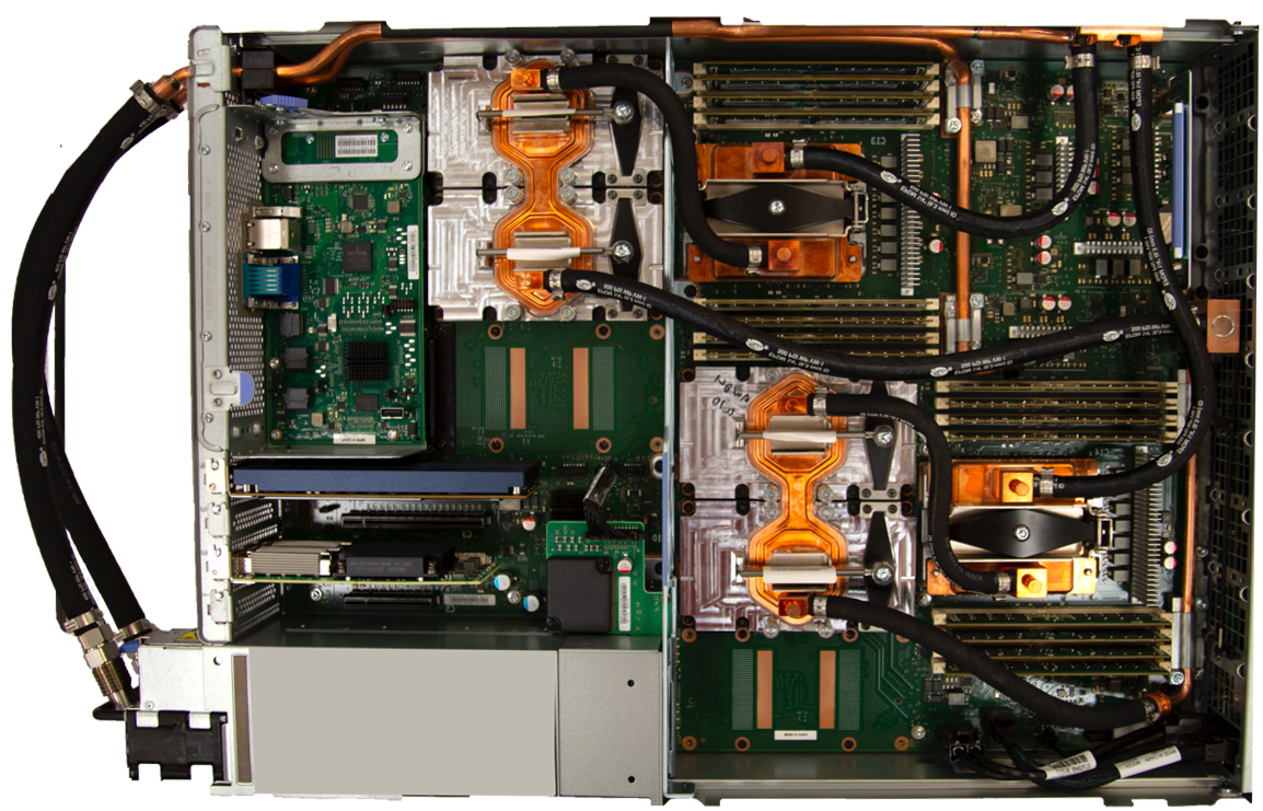
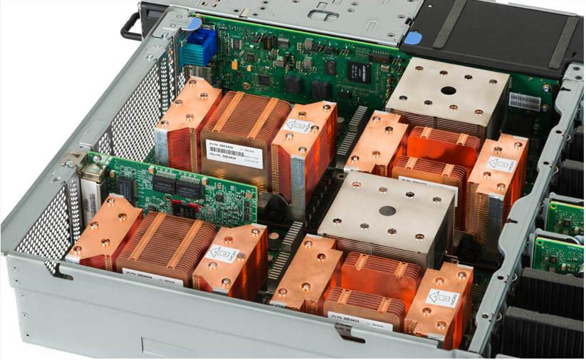
- Images (click for larger image)
- Sierra POWER9 AC922 compute node and its primary components. Relevant individual components are discussed in more detail in sections below.
- Sierra POWER9 AC922 node diagram. (Adapted from: "IBM Power System AC922 Introduction and Technical Overview". IBM Redpaper publication REDP-5472-00 by Alexandre Bicas Caldeira. March, 2018)

POWER9 Processor Key Characteristics
- IBM 14 nm Silicon-On-Insulator (SOI) technology; 8 billion transistors
- IBM offers POWER9 in two different designs: Scale-Out and Scale-Up
- Scale-Out:
- Designed for traditional datacenter clusters utilizing single-socket and dual-socket servers.
- Optimized for Linux servers
- 24-core and 12-core models
- Scale-Up:
- Designed for NUMA servers with four or more sockets, supporting large amounts of memory capacity and throughput.
- Optimized for PowerVM servers
- 24-core and 12-core models
- Core variants: Some POWER9 models vary the number of active cores and have 16, 18, 20 or 22 cores. LLNL's AC922 compute nodes use 22 cores.
- Hardware threads:
- 12-core processors are SMT8 (8 hardware threads/core)
- 24-core processors are SMT4 (4 hardware threads/core).
- L1 data cache: 32 KB per core, 8-way, private
- L1 instruction cache: 32 KB per core, 8-way, private
- L2 cache: 512 KB per core (SMT8), 512 KB per core pair (SMT4), 8-way, private
- L3 cache: 120 MB, 20-way, shared as twelve 10 MB banks
- Clock: due to adaptive power management options, the clock speed can vary depending upon the system load. At LC speeds can vary from approximately 2.3 - 3.8 GHz. LC can also set the clock to a specific speed regardless of workload.
- High-throughput on-chip fabric: Over 7 TB/s aggregate bandwidth via on-chip switch connecting cores to memory, PCIe, GPUs, etc.
- Images:
- Schematics of the POWER9 processor chip variants are shown below. Click for a larger version. (Source: "POWER9 Processor for the Cognitive Era". IBM presentation by Brian Thompto. Hot Chips 28 Symposium, October 2016)

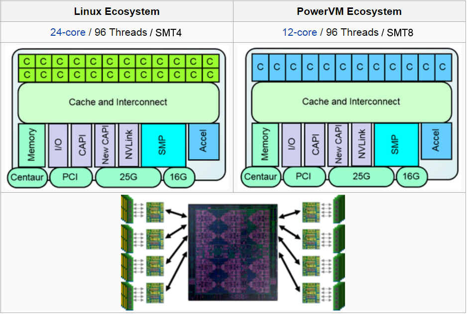
- Images of the POWER9 processor chip die are shown below. Click for a larger version. (Source: "POWER9 Processor for the Cognitive Era". IBM presentation by Brian Thompto. Hot Chips 28 Symposium, October 2016)


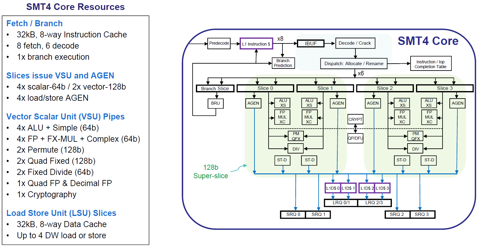
POWER9 Core Key Features
- The POWER9 processor core is a 64-bit implementation of the IBM Power Instruction Set Architecture (ISA) Version 3.0
- Little Endian
- 8-way (SMT8) or 4-way (SMT4) hardware threads
- Basic building block of both SMT4 and SMT8 cores is a slice:
- A slice is a rudimentary 64-bit single threaded processing element with a load store unit (LSU), integer unit (ALU) and vector scalar unit (VSU, doing SIMD and floating point).
- Two slices are combined to make a 128-bit "super-slice"
- Both SMT4 and SMT8 cores contain the same number of slices (threads) = 96.
- Shorter fetch-to-compute pipeline than POWER8; reduced by 5 cycles.
- Instructions per cycle: 128 for SMT8, 64 for SMT4
- Images:
- Schematic of a POWER9 SMT4 core is shown below. Click for a larger version. (Source: "POWER9 Processor for the Cognitive Era". IBM presentation by Brian Thompto. Hot Chips 28 Symposium, October 2016)
References and More Information:
- "POWER9 Processor for the Cognitive Era". IBM presentation by Brian Thompto. Hot Chips 28 Symposium, October 2016
- "POWER9 - Microarchitectures - IBM". wikichip.org website.
- "Regaining America's Supercomputing Supremacy with the Summit Supercomputer". Paul Alcorn on the tomshardware.com website, November 20, 2017.
- "POWER9 to the People". Timothy Prickett Morgan on the nextplatform.com website, December 5, 2017.
NVIDIA Tesla P100 (Pascal) Architecture
Used by LLNL's Early Access systems ray, rzmanta, shark
Tesla P100 Key Features
- "Extreme performance" for HPC and Deep Learning:
- 5.3 TFLOPS of double-precision floating point (FP64) performance
- 10.6 TFLOPS of single-precision (FP32) performance
- 21.2 TFLOPS of half-precision (FP16) performance
- NVLink: NVIDIA's high speed, high bandwidth interconnect
- Connects multiple GPUs to each other, and GPUs to the CPUs
- 4 NVLinks per GPU
- Up to 160 GB/s bidirectional bandwidth between GPUs (5x the bandwidth of PCIe Gen 3 x16)
- HBM2: High Bandwidth Memory 2
- Memory is located on same physical package as the GPU, providing 3x the bandwidth of previous GPUs such as the Maxwell GM200
- Highly tuned 16 GB HBM2 memory subsystem delivers 732 GB/sec peak memory bandwidth on Pascal.
- Unified Memory:
- Significant advancement and a major new hardware and software-based feature of the Pascal GP100 GPU architecture.
- First NVIDIA GPU to support hardware page faulting, and when combined with new 49-bit (512 TB) virtual addressing, allows transparent migration of data between the full virtual address spaces of both the GPU and CPU.
- Provides a single, seamless unified virtual address space for CPU and GPU memory.
- Greatly simplifies GPU programming - programmers no longer need to manage data sharing between two different virtual memory systems.
- Compute Preemption:
- New hardware and software feature that allows compute tasks to be preempted at instruction-level granularity.
- Prevents long-running applications from either monopolizing the system or timing out. For example, both interactive graphics tasks and interactive debuggers can run simultaneously with long-running compute tasks.
- Images:
- NVIDIA Tesla P100 with Pascal GP100 GPU. Click for larger image. (Source: NVIDIA Tesla P100 Whitepaper. NVIDIA publication WP-08019-001_v01.1. 2016)
- IBM Power System S822LC with two IBM POWER8 CPUs and four NVIDIA Tesla P100 GPUs connected via NVLink. Click for larger image.
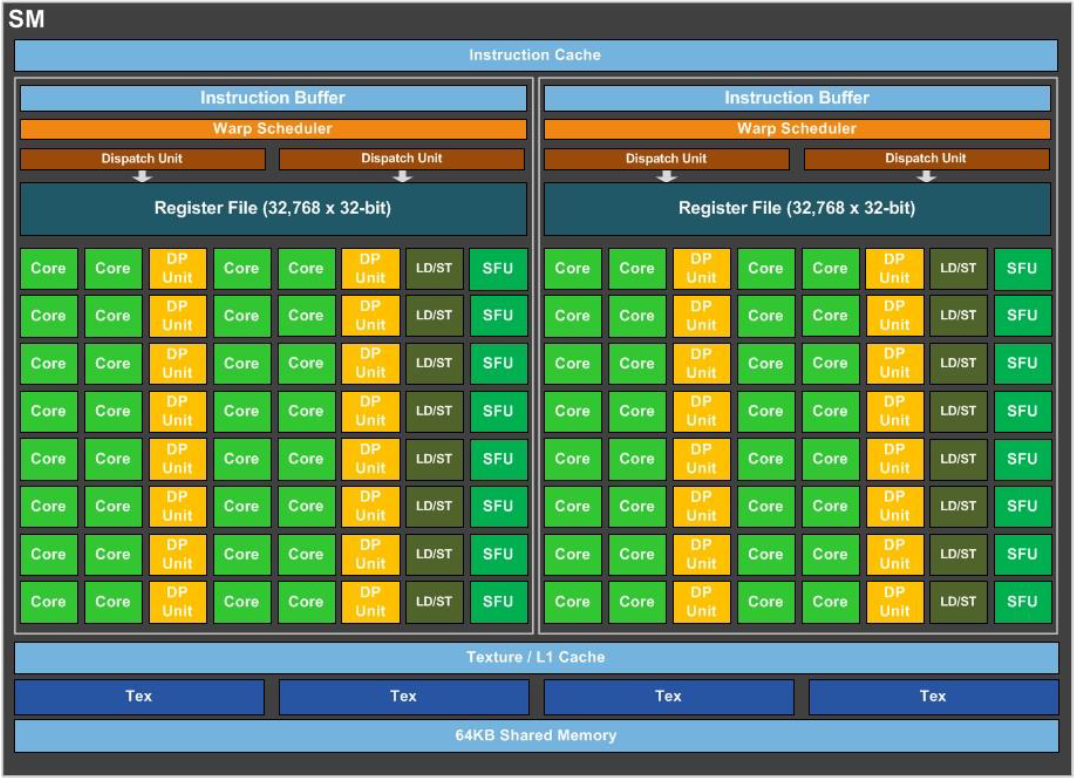
Pascal GP100 GPU Components
- A full GP100 includes 6 Graphics Processing Clusters (GPC)
- Each GPC has 10 Pascal Streaming Multiprocessors (SM) for a total of 60 SMs
- Each SM has:
- 64 single-precision CUDA cores for a total of 3840 single-precision cores
- 4 Texture Units for a total of 240 texture units
- 32 double-precision units for a total of 1920 double-precision units
- 16 load/store units, 16 special function units, register files, instruction buffers and cache, warp schedulers and dispatch units
- L2 cache size of 4096 KB
- Note The Tesla P100 does not use a full Pascal GP100. It uses 56 SMs instead of 60, for a total core count of 3584
- Images:
- Diagrams of a full Pascal GP100 GPU and a single SM. Click for larger image. (Source: NVIDIA Tesla P100 Whitepaper. NVIDIA publication WP-08019-001_v01.1. 2016)

References and More Information
- NVIDIA Whitepaper: "NVIDIA Tesla P100". Publication WP-08019-001_v01.1. 2016.
- NVIDIA developers blog: "Inside Pascal: NVIDIA's Newest Computing Platform" by Mark Harris, NVIDIA. June 19, 2016.
NVIDIA Tesla V100 (Volta) Architecture
Used by LLNL's Sierra systems sierra, lassen, rzansel
Tesla P100 Key Features
- New Streaming Multiprocessor (SM) Architecture Optimized for Deep Learning:
- 50% more energy efficient than the previous generation Pascal design, enabling major boosts in FP32 and FP64 performance in the same power envelope.
- Tensor Cores designed specifically for deep learning deliver up to 12x higher peak TFLOPS for training and 6x higher peak TFLOPS for inference.
- With independent parallel integer and floating-point data paths, the Volta SM is also much more efficient on workloads with a mix of computation and addressing calculations.
- Independent thread scheduling capability enables finer-grain synchronization and cooperation between parallel threads.
- Combined L1 data cache and shared memory unit significantly improves performance while also simplifying programming.
- Performance:
- 7.8 TFLOPS of double-precision floating point (FP64) performance
- 15.7 TFLOPS of single-precision (FP32) performance
- 125 Tensor TFLOPS
- Second-Generation NVIDIA NVLink:
- Delivers higher bandwidth, more links, and improved scalability for multi-GPU and multi-GPU/CPU system configurations.
- Supports up to six NVLink links and total bandwidth of 300 GB/sec, compared to four NVLink links and 160 GB/s total bandwidth on Pascal.
- Now supports CPU mastering and cache coherence capabilities with IBM Power 9 CPU-based servers.
- The new NVIDIA DGX-1 with V100 AI supercomputer uses NVLink to deliver greater scalability for ultra-fast deep learning training.
- HBM2 Memory: Faster, Higher Efficiency
- Highly tuned 16 GB HBM2 memory subsystem delivers 900 GB/sec peak memory bandwidth.
- The combination of both a new generation HBM2 memory from Samsung, and a new generation memory controller in Volta, provides 1.5x delivered memory bandwidth versus Pascal GP100, with up to 95% memory bandwidth utilization running many workloads.
- Volta Multi-Process Service (MPS):
- Enables multiple compute applications to share GPUs.
- Volta MPS also triples the maximum number of MPS clients from 16 on Pascal to 48 on Volta.
- Enhanced Unified Memory and Address Translation Services:
- Provides a single, seamless unified virtual address space for CPU and GPU memory.
- Greatly simplifies GPU programming - programmers no longer need to manage data sharing between two different virtual memory systems.
- Includes new access counters to allow more accurate migration of memory pages to the processor that accesses them most frequently, improving efficiency for memory ranges shared between processors.
- On IBM Power platforms, new Address Translation Services (ATS) support allows the GPU to access the CPU's page tables directly.
- Maximum Performance and Maximum Efficiency Modes:
- In Maximum Performance mode, the Tesla V100 accelerator will operate up to its TDP (Thermal Design Power) level of 300 W to accelerate applications that require the fastest computational speed and highest data throughput.
- Maximum Efficiency Mode allows data center managers to tune power usage of their Tesla V100 accelerators to operate with optimal performance per watt. A not-to-exceed power cap can be set across all GPUs in a rack, reducing power consumption dramatically, while still obtaining excellent rack performance.
- Cooperative Groups and New Cooperative Launch APIs:
- Cooperative Groups is a new programming model introduced in CUDA 9 for organizing groups of communicating threads.
- Allows developers to express the granularity at which threads are communicating, helping them to express richer, more efficient parallel decompositions.
- Basic Cooperative Groups functionality is supported on all NVIDIA GPUs since Kepler. Pascal and Volta include support for new cooperative launch APIs that support synchronization amongst CUDA thread blocks. Volta adds support for new synchronization patterns.
- Volta Optimized Software:
- New versions of deep learning frameworks such as Caffe2, MXNet, CNTK, TensorFlow, and others harness the performance of Volta to deliver dramatically faster training times and higher multi-node training performance.
- Volta-optimized versions of GPU accelerated libraries such as cuDNN, cuBLAS, and TensorRT leverage the new features of the Volta GV100 architecture to deliver higher performance for both deep learning inference and High Performance Computing (HPC) applications.
- The NVIDIA CUDA Toolkit version 9.0 includes new APIs and support for Volta features to provide even easier programmability.
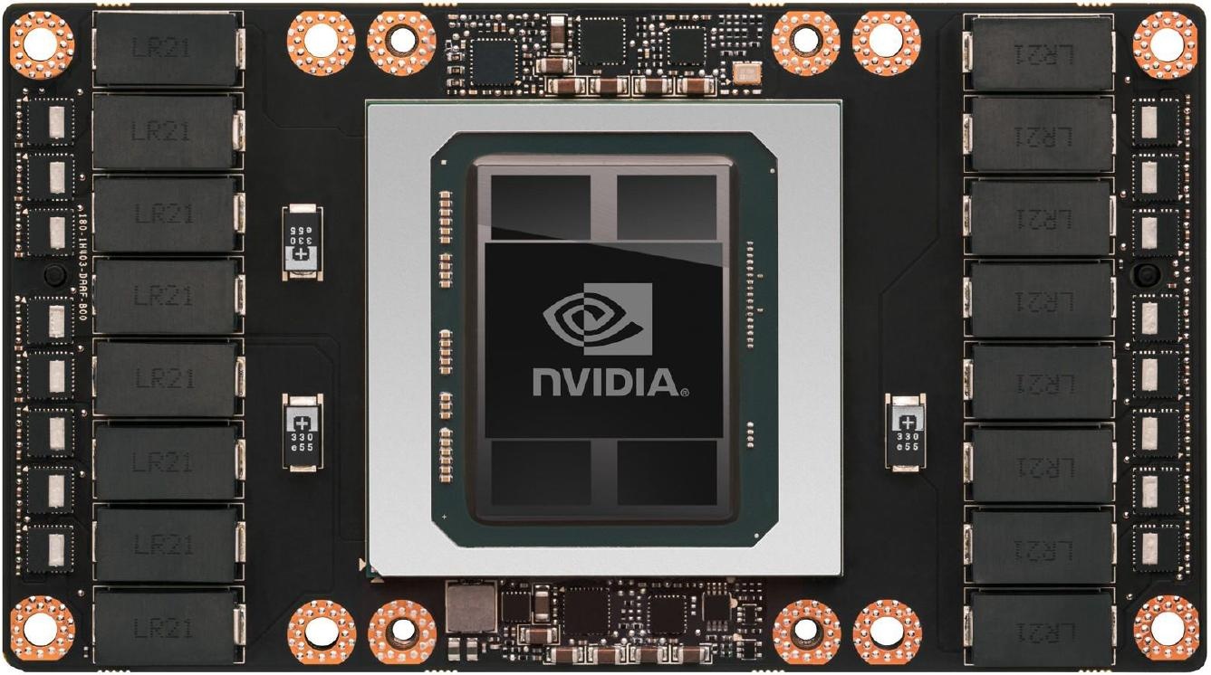
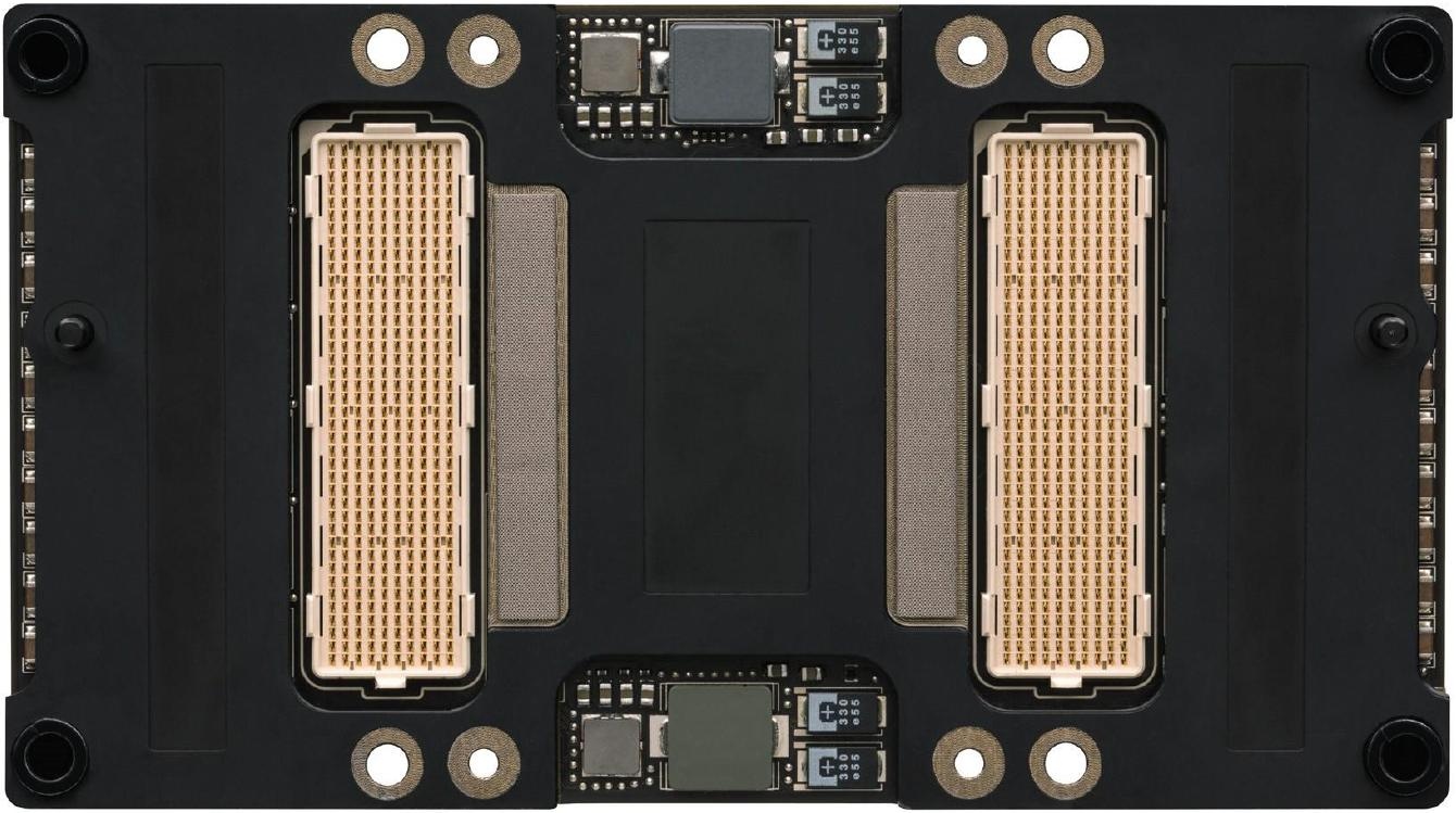
- Images:
- NVIDIA Tesla V100 with Volta GV100 GPU. Click for larger image. (Source: NVIDIA Tesla V100 Whitepaper. NVIDIA publication WP-08608-001_v1.1. August 2017)


- IBM Power System AC922 with two IBM POWER9 CPUs and four NVIDIA Tesla V100 GPUs connected via NVLink.
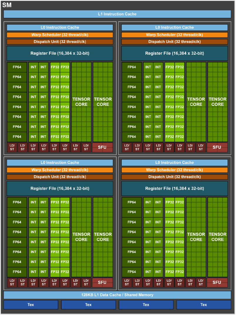
Volta GV100 GPU Components
- A full GV100 includes 6 Graphics Processing Clusters (GPC)
- Each GPC has 14 Volta Streaming Multiprocessors (SM) for a total of 84 SMs
- Each SM has:
- 64 single-precision floating-point cores; GPU total of 5376
- 64 single-precision integer cores; GPU total of 5376
- 32 double-precision floating-point cores; GPU total of 2688
- 8 Tensor Cores; GPU total of 672
- 4 Texture Units; GPU total of 168
- 32 load/store units, 4 special function units, register files, instruction buffers and cache, warp schedulers and dispatch units
- L2 cache size of 6144 KB
- Note The Tesla V100 does not use a full Volta GV100. It uses 80 SMs instead of 84, for a total "CUDA" core count of 5120 versus 5376.
- Images:
- Diagrams of a full Volta GV100 GPU and a single SM. Click for larger image. (Source: NVIDIA Tesla V100 Whitepaper. NVIDIA publication WP-08608-001_v1.1. August 2017)

References and More Information
- NVIDIA Whitepaper: "NVIDIA Tesla V100 GPU Architecture". Publication WP-08608-001_v1.1. August 2017.
- NVIDIA developers blog: "Inside Volta: The World's Most Advanced Data Center GPU" by Luke Durant, Olivier Giroux, Mark Harris and Nick Stam, NVIDIA. May 10, 2017.
NVLink
- NVLink is NVIDIA's high-speed interconnect technology for GPU accelerated computing. Used to connect GPUs to GPUs and/or GPUs to CPUs.
- Significantly increases performance for both GPU-to-GPU and GPU-to-CPU communications.
- NVLink - first generation
- Debuted with Pascal GPUs
- Used on LC's Early Access systems (ray, rzmanta, shark)
- Supports up to 4 NVLink links per GPU.
- Each link provides a 40 GB/s bidirectional connection to another GPU or a CPU, yielding an aggregate bandwidth of 160 GB/s.
- NVLink 2.0 - second generation
- Debuted with Volta GPUs
- Used on LC's Sierra systems (sierra, lassen, rzansel)
- Supports up to 6 NVLink links per GPU.
- Each link provides a 50 GB/s bidirectional connection to another GPU or a CPU, yielding an aggregate bandwidth of 300 GB/s.
- Multiple links can be "ganged" to increase bandwidth between two endpoints
- Numerous NVLink topologies are possible, and different configurations can be optimized for different applications.
- LC's NVLink configurations:
- Early Access systems (ray, rzmanta, shark): Each CPU is connected to 2 GPUs by 2 NVLinks each. Those GPUs are connected to each other by 2 NVLinks each
- Sierra systems (sierra, lassen, rzansel): Each CPU is connected to 2 GPUs by 3 NVLinks each. Those GPUs are connected to each other by 3 NVLinks each
- GPUs on different CPUs do not connect to each other with NVLinks
- Images:
- Two representative NVLink 2.0 topologies are shown below. (Source: NVIDIA Tesla V100 Whitepaper. NVIDIA publication WP-08608-001_v1.1. August 2017)
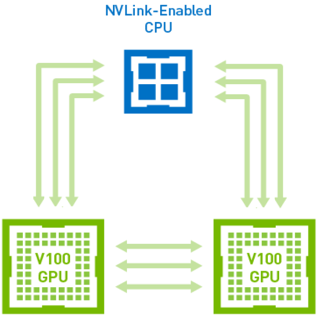
(LC's Sierra systems)

References and More Information
- NVIDIA Whitepaper: "NVIDIA Tesla V100 GPU Architecture". Publication WP-08608-001_v1.1. August 2017.
- NVIDIA Whitepaper: "NVIDIA Tesla P100". Publication WP-08019-001_v01.1. 2016.
Mellanox EDR InfiniBand Network
Hardware
- Mellanox EDR InfiniBand is used for both Early Access and Sierra systems:
- EDR = Enhanced Data Rate
- 100 Gb/s bandwidth rating
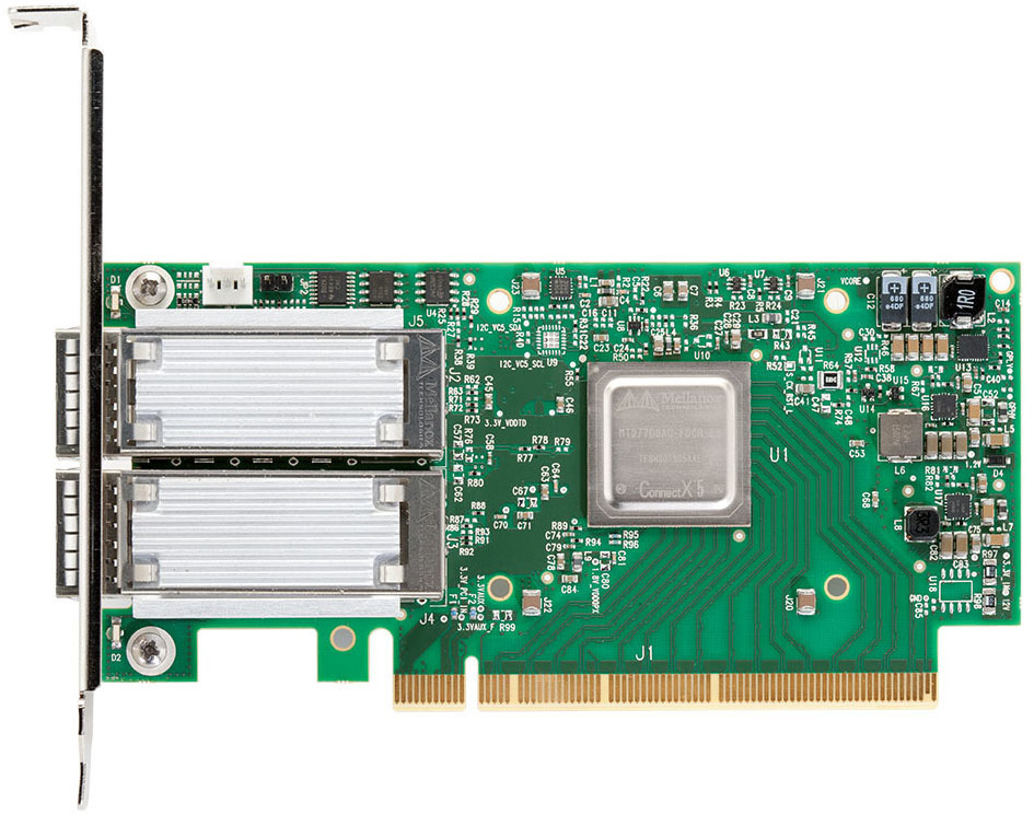
- Adapters:
- Nodes have one dual-port Mellanox ConnectX EDR InfiniBand adapter (at LC)
- Both PCIe Gen 3.0 and Gen 4.0 capable
- Adapter ports connect to level 1 switches
- Top-of-Rack (TOR) level 1 (edge) switches:
- Mellanox Switch-IB with 36 ports
- Down ports connect to node adapters
- Up ports connect to level 2 switches
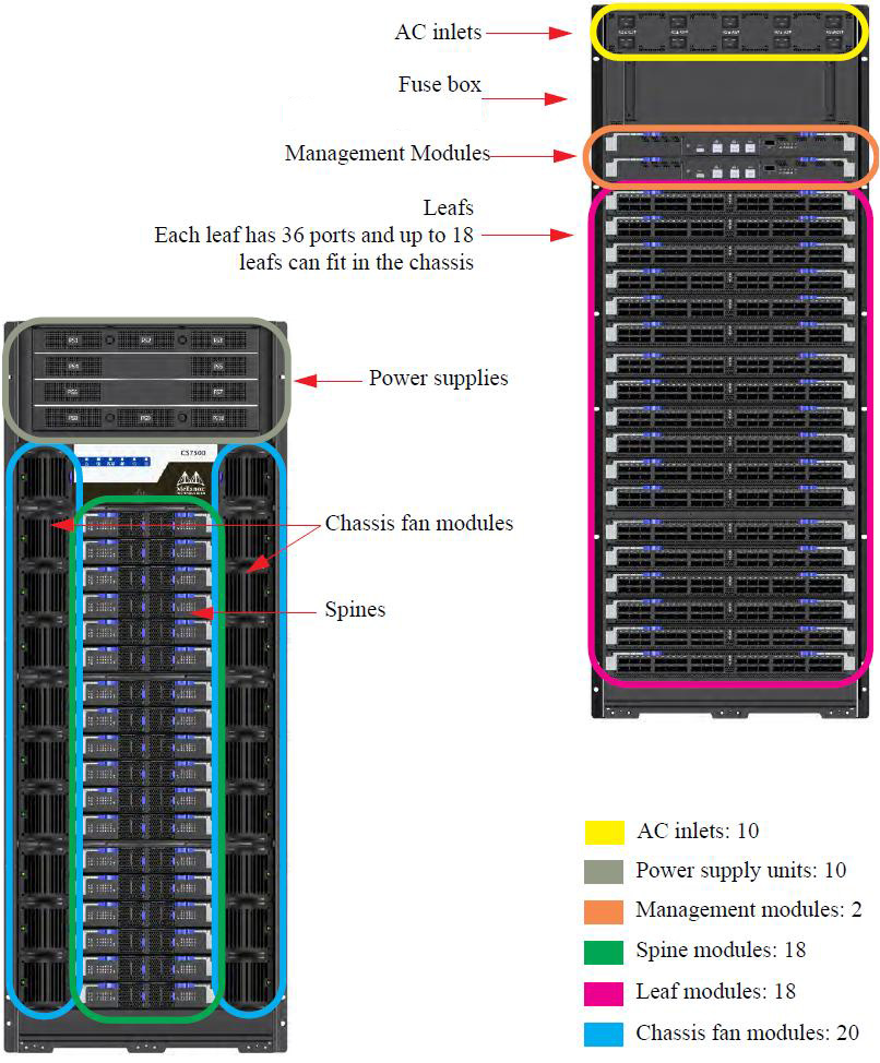
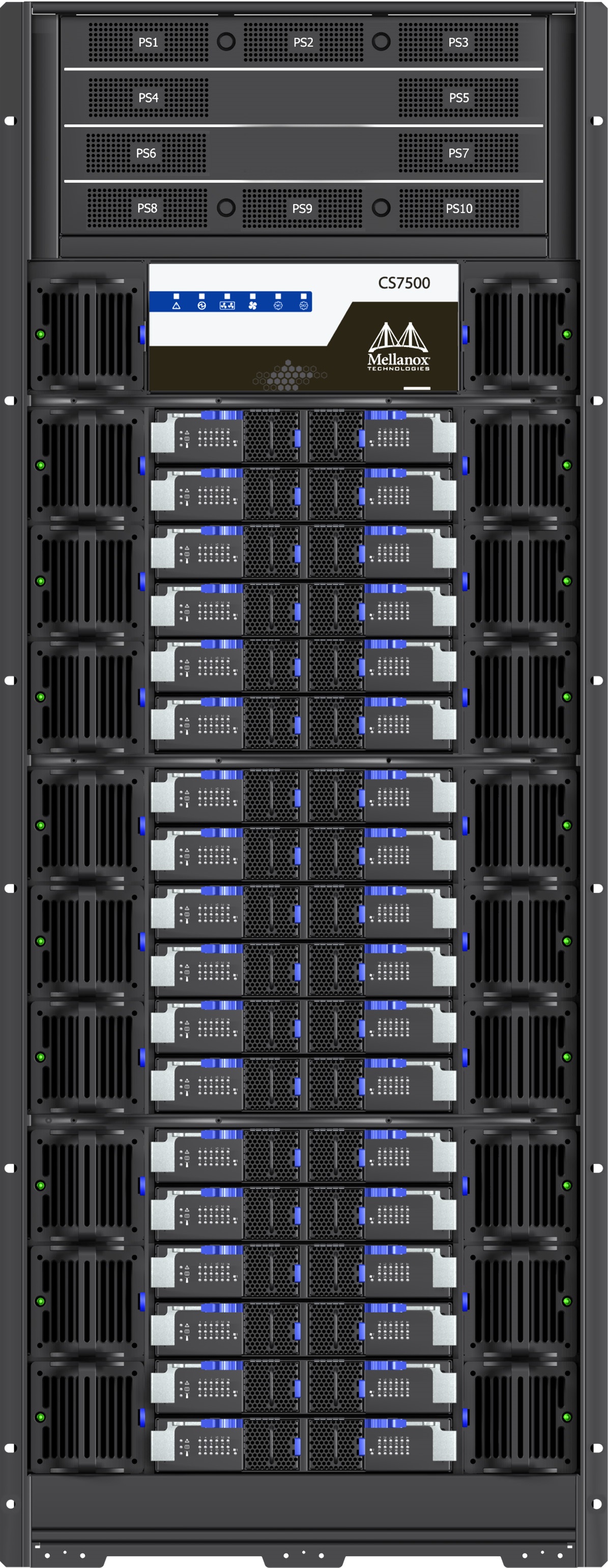
- Director level 2 (core) switches:
- Mellanox CS7500 with 648 ports
- Holds 18 Mellanox Switch-IB 36-port leafs
- Ports connect down to level 1 switches
- Images:
- Mellanox EDR InfiniBand network hardware components are shown below. Click for larger image. (Source: mellanox.com)

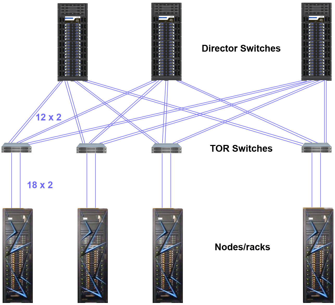
Topology and LC Sierra Configuration
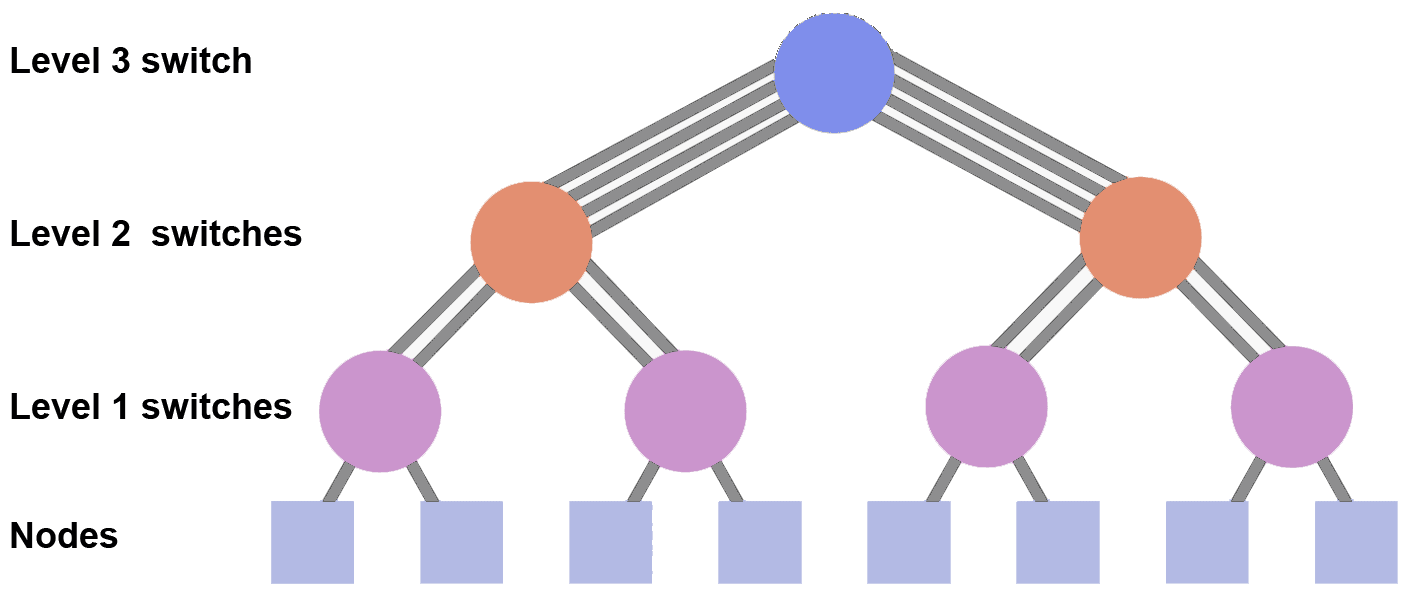
- Tapered Fat Tree, Single Plane Topology
- Fat Tree: switches form a hierarchy with higher level switches having more (hence, fat) connections down than lower level switches.
- Tapered: the number of connections down for lower level switches are increased by a ratio of two-to-one.
- Single Plane: nodes connect to a single fat tree network.
- Sierra configuration details:
- Each rack has 18 nodes and 2 TOR switches
- Each node's dual-port adapter connects to both of its rack's TOR switches with one port each. That equals 18 uplinks to each TOR within a rack.
- Each TOR switch has 12 uplinks to Director switches, at least one per Director switch
- There are 9 Director switches
- Because each TOR switch has 12 uplinks and there are only 9 Director switches, there are 3 extra uplinks per TOR switch. These are used to connect twice to 3 of the 9 Director switches.
- Note Sierra has a "modified" 2:1 Tapered Fat Tree. It's actually 1.5 to 1 (18 links down, 12 links up for each TOR switch).
- At LC, adapters connect to level 1 switches via copper cable. Level 1 switches connect to level 2 switches via optic fiber.
- Images:
- Topology diagrams shown below. Click for larger image.
References and More Information
- Mellanox CS7500 InfiniBand Switch Brochure. Mellanox Technologies 2017.
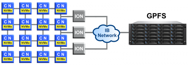
NVMe PCIe SSD (Burst Buffer)
- NVMe PCIe SSD:
- SSD = Solid State Drive; non-volatile storage device with no moving parts
- PCIe = Peripheral Component Interconnect Express; standard high-speed serial bus connection.
- NVMe = Non-Volatile Memory Express; device interface specification for accessing non-volatile storage media attached via PCIe bus
- Fast and intermediate storage layer positioned between the front-end computing processes and the back-end storage systems.
- Primary purpose of this fast storage is to act as a "Burst Buffer" for improving I/O performance. Computation can continue while the fast SSD "holds" data (such as checkpoint files) being written to slower disk.
-
Mounted as a file system local to a compute node (not global storage).
- Sierra systems (sierra, lassen, rzansel):
- Compute nodes have 1.6 TB SSD.
- The login and launch nodes also have this SSD, but from a user perspective, it's not really usable.
- Managed via the LSF scheduler.
- CORAL Early Access systems:
- Ray compute nodes have 1.6 TB SSD. The shark and rzmanta systems do not have SSD.
- Mounted under /l/nvme (lower case "L" / nvme)
- Users can write/read directly to this location
- Unlike Sierra systems, it is not managed via LSF
- As with all SSDs, life span is shortened with writes
-
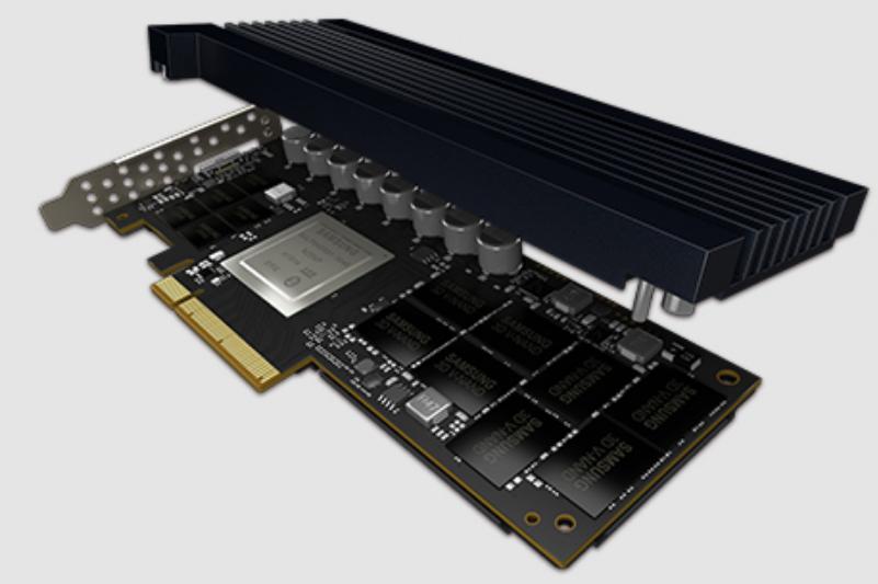
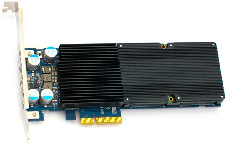
Performance: the Samsung literature (see References below) cites different performance numbers for the SSD used in Sierra systems. Both are shown below:
Samsung PM1725a brochure Samsung PM1725a data sheet 6400 MB/s Sequential Read BW 5840 MB/s Sequential Read BW 3000 MB/s Sequential Write BW 2100 MB/s Sequential Write BW 1080K IOPS Random Read 1000K IOPS Random Read 170K IOPS Random Write 140K IOPS Random Write - Usage information:
- See the Burst Buffer Usage section of this tutorial
- Sierra confluence wiki: https://lc.llnl.gov/confluence/display/SIERRA/Burst+Buffers.
- Images:
- 1.6 TB NVMe PCIe SSD. Click for larger image. (Sources: samsung.com and hgst.com)


References and More Information
- Samsung PM1725 Brochure. SSD used on Sierra systems.
- Samsung 1.6TB HHHL PM1725a data sheet: http://www.samsung.com/semiconductor/ssd/enterprise-ssd/MZPLL1T6HEHP/
- HGST Ultrastar SN100 Data Sheet. SSD used on the Ray system.
Accounts, Allocations and Banks
Accounts
- Only a brief summary of LC account request procedures is included below. For details, see: https://hpc.llnl.gov/accounts
- Sierra:
- Sierra is considered a Tri-lab Advanced Technology System (ATS).
- Accounts on the classified sierra system are restricted to approved Tri-lab (LLNL, LANL, SNL) users.
- Guided by the ASC Advanced Technology Computing Campaign (ATCC) proposal process and usage model.
- Accounts for the other Sierra systems (lassen, rzansel) and Early Access systems (ray, shark, rzmanta) follow the usual account request processes, summarized below.
- LLNL and Collaborators:
- Go to https://lc-idm.llnl.gov
- OCF resource: lassen, rzansel, ray, rzmanta
- SCF resource: shark
- LANL and Sandia:
- Go to https://sarape.sandia.gov
- LLNL resources: lassen, rzansel, ray, rzmanta and shark (depending on clearance/citizenship)
- Sponsor: Greg Tomaschke, tomaschke1@llnl.gov, 925-423-0561
- PSAAP centers:
- Go to https://sarape.sandia.gov
- LLNL resources: lassen, ray
- Sponsor: Tim Fahey
- For any questions or problems regarding accounts, please contact the LC Hotline account specialists:
- Email: lc-support.llnl.gov
- Phone: 925-422-4533
Allocations and Banks
- Sierra allocations and banks follow the ASC Advanced Technology Computing Campaign (ATCC) proposal process and usage model
- Approved ATCC proposals are provided with an atcc bank / allocation
- Additionally, ASC executive discretionary banks (lanlexec, llnlexec and snlexec) are provided for important Tri-lab work not falling explicitly under an ATCC proposal.
- Lassen is similar to other LC systems - users need to be in a valid "bank" in order to run jobs.
- Rzansel and the CORAL EA systems currently use a "guests" group/bank for most users.
Bank-Related Commands
- IBM's Spectrum LSF software is used to schedule/manage jobs run on all Sierra systems. LSF is very different than Slurm used on other LC systems.
- Familiar Slurm commands for getting bank and usage information are not available.
- The most useful command to obtain bank allocation and usage information is the LC developed lshare command.
- The lshare command and several other related commands are discussed in the Banks, Job Usage and Job History Information section of this tutorial.
Accessing LC's Sierra Machines
- The instructions below summarize the basics for connecting to LC's Sierra systems. Additional access related information can be found at:
- LLNL: https://hpc.llnl.gov/manuals/access-lc-systems.
- LANL: https://hpc.lanl.gov/networks/red-network/red-network-tri-lab-user-access.html (requires LANL authentication)
- Sandia: https://hpc.sandia.gov/access/index.html
- SSH (version 2) is used to connect to all LC machines:
- From a terminal window command line, simply ssh machinename, where machinename is the name of the cluster.
- SSH keys can be used between LC machines only. Instructions can be found at: /documentation/user-guides/accessing-lc-systems#setting-up-ssh-keys
- Additional SSH details can be found at https://hpc.llnl.gov/training/tutorials/livermore-computing-resources-and-environment#ssh

- RSA tokens are used for authentication:
- Static 4-8 character PIN + 6 digits from token
- There is one token for the CZ and SCF, and one token for the RZ.
- Sandia / LANL Tri-lab logins can be done without tokens
- Machine names and login nodes:
- Each system has a single cluster login name, such as sierra, lassen, ray, etc.
- A full llnl.gov domain name is required if coming from outside LLNL.
- Successfully logging into the cluster will place you on one of the available login nodes.
- User logins are distributed across login nodes for load balancing.
- To view available login nodes use the nodeattr -c login command.
- You can ssh from one login node to another, which may be useful if there are problems with the login node you are on.
- X11 Forwarding
- In order to display GUIs back to your local workstation, your SSH session will need to have X11 Forwarding enabled.
- This is easily done by including the -X (uppercase X) or -Y option with your ssh command. For example: ssh -X sierra.llnl.gov
- Your local workstation will also need to have X server software running. This comes with Linux by default. For Macs, something like XQuartz (http://www.xquartz.org/) can be used. For Windows, there are several options - LLNL provides X-Win32 with a site license.
- SSH Clients
- Used instead of a terminal window SSH command - mostly applies to Windows machines.
- You will need to follow the instructions for your specific client.
- Instructions for using X-Win32, provided by LLNL, can be found at: /documentation/user-guides/accessing-lc-systems#connection-to-LC-machines-with-x-win32
How to Connect
- Use the table below to connect to LC's Sierra systems.
| Going to ↓ Coming from → | LLNL | LANL/Sandia | Other/Internet |
|---|---|---|---|
|
SCF sierra |
|
|
|
|
OCF-CZ lassen |
|
|
|
|
OCF-RZ rzansel |
|
**Note: Effective Aug 2019** |
|
Software and Development Environment
Similarities and Differences
- The Sierra software and development environment is similar in a number of ways to LC's other production clusters. Common topics are briefly discussed below, and covered in more detail in the Introduction to LC Resources tutorial.
- Sierra systems are also very different from other LC systems in important ways. These differences are summarized below and covered in detail later in other sections.
Login Nodes
- Each LC cluster has a single, unique hostname used for login connections. This is called the "cluster login".
- The cluster login is actually an alias for the real login nodes. It "rotates" logins between the actual login nodes for load balancing purposes.
- For example: sierra.llnl.gov is the cluster login which distributes user logins over any number of physical login nodes.
- The number of physical login nodes on any given LC cluster varies.
- Login nodes are where you perform interactive, non-cpu intensive work: launch tools, edit files, submit batch jobs, run interactive jobs, etc.
- Shared by multiple users
- Should not be used to run production or parallel jobs, or perform long running parallel compiles/builds. These activities can impact other users.
- Users don't need to know (in most cases) the actual login node they are rotated onto - unless there are problems. Using the hostname command will indicate the actual login node name for support purposes.
- If the login node you are on is having problems, you can ssh directly to another one. To find the list of available login nodes, use the command: nodeattr -c login
- Cross-compilation is not necessary on Sierra clusters because login nodes have the same architecture as compute nodes.
Launch Nodes
- In addition to login nodes, Sierra systems have a set of nodes that are dedicated to launching and managing user jobs. These are called launch nodes.
- Typically, users submit jobs from a login node:
- Batch jobs: a job script is submitted with the bsub command
- Interactive jobs: a shell or xterm session is requested using the bsub or lalloc commands
- The job is then migrated to a launch node where LSF takes over. An allocation of compute node(s) is acquired.
- Finally, the job is started on the compute node allocation
- If it's a parallel job using the jsrun command the parallel tasks will run on these nodes
- Serial jobs and the actual job command script will run on the first compute node as a "private launch node" (by default at LC)
- Further details on launch nodes are discussed as relevant in the Running Jobs Section.
Login Shells and Files
- Your login shell is established when your LC account is initially setup. The usual login shells are supported:
/bin/bash
/bin/csh
/bin/ksh
/bin/sh
/bin/tcsh
/bin/zsh - All LC users automatically receive a set of login files. These include:
.cshrc .kshenv .login .profile
.kshrc .logout
.cshrc.linux .kshrc.linux .login.linux .profile.linux
- Which files are of interest depend upon your shell
- Note for bash and zsh users: LC does not provide .bashrc, .bash_profile, .zprofile or .zshrc files at this time.
- These files and usage details are further discussed at: https://hpc.llnl.gov/training/tutorials/livermore-computing-resources-and-environment#HomeDirectories.
Operating System
- Sierra systems run Red Hat Enterprise Linux (RHEL). The current version can be determined by using the command: cat /etc/redhat-release
- Although they do not run the standard TOSS stack like other LC Linux clusters, LC has implemented some TOSS configurations, such as using /usr/tce instead of /usr/local.
Batch System
- Unlike most other LC clusters, Sierra systems do NOT use Slurm as their workload manager / batch system.
- IBM's Platform LSF Batch System software is used to schedule/manage jobs run on all Sierra systems.
- LSF is very different from Slurm:
- Will require a bit of a learning curve for new users.
- Existing job scripts will require modification.
- Other scripts using Slurm commands will also require modification
- LSF is discussed in detail in the Running Jobs Section of this tutorial.
File Systems
- Sierra systems mount the usual LC file systems.
- The only significant differences are:
- Parallel file systems: IBM's Spectrum Scale product is used instead of Lustre.
- NVMe SSD (burst buffer) storage is available
- Available file systems are summarized in the table below and discussed in more detail in the File Systems Section of the Livermore Computing Resources and Environment tutorial.
| File System | Mount Points | Backed Up? | Purged? | Comments |
|---|---|---|---|---|
| Home directories | /g/g0 - /g/g99 | Yes | No | 24 GB quota; safest file system; includes .snapshot directory for online backups |
| Workspace | /usr/workspace/ws | No | No | 1 TB quota for each user and each group; includes .snapshot directory for online backups |
| Local tmp | /tmp /usr/tmp /var/tmp |
No | Yes | Node local temporary file space; small; actually resides in node memory, not physical disk |
| Collaboration | /usr/gapps /usr/gdata /collab/usr/gapps /collab/usr/gdata |
Yes | No | User managed application directories; intended for collaborative development and usage |
| Parallel | /p/gpfs1 |
No | Yes | Intended for parallel I/O; large, shared by all users on a cluster. IBM's Spectrum Scale (not Lustre). Mounted as /p/gpfs1 on sierra, lassen and rzansel. |
| Burst buffer | $BBPATH | No | Yes | Each node has a 1.6 TB NVMe PCIe SSD. Available only when requested through bsub. See NVMe PCIe SSD (Burst Buffer) for details. For CORAL EA systems, only ray compute nodes have the 1.6 TB NVMe, and it is statically mounted under /l/nvme. |
| HPSS archival storage | server based | No | No | Virtually unlimited archival storage; accessed by "ftp storage" from LC machines. |
| FIS | server based | No | Yes | File Interchange System; for transferring files between unclassified/classified networks |
HPSS Storage
- As with all other production LC systems, Sierra systems have access to LC's High Performance Storage System (HPSS) archival storage.
- The HPSS system is named storage.llnl.gov on both the OCF and SCF.
- LC does not backup temporary file systems, including the scratch parallel file systems. Users should backup their important files to storage.
- Several different file transfer tools are available.
- See https://hpc.llnl.gov/training/tutorials/livermore-computing-resources-and-environment#Archival for details on using HPSS storage.
Modules
- As with LC's TOSS 3 systems, Lmod modules are used for most software packages, such as compilers, MPI and tools.
- Dotkits are no longer used.
- Users only need to know a few commands to effectively use modules - see the table below.
- Note The "ml" shorthand can be used instead of "module" - for example: "ml avail"
- See Using https://hpc.llnl.gov/software/modules-and-software-packaging for more information.
| Command | Shorthand | Description |
|---|---|---|
| module avail | ml avail | List available modules |
| module load package | ml load package | Load a selected module |
| module list | ml | Show modules currently loaded |
| module unload package | ml unload package | Unload a previously loaded module |
| module purge | ml purge | Unload all loaded modules |
| module reset | ml reset | Reset loaded modules to system defaults |
| module update | ml update | Reload all currently loaded modules |
| module display package | n/a | Display the contents of a selected module |
| module spider | ml spider | List all modules (not just available ones) |
| module keyword key | ml keyword key | Search for available modules by keyword |
| module module help |
ml keyword key | Display module help |
Compilers Supported
- The following compilers are available and supported on LC's Sierra systems:
| Compiler | Description |
|---|---|
| XL | IBM's XL C/C++ and Fortran compilers |
| Clang | IBM's C/C++ clang compiler |
| GNU | GNU compiler collection, C, C++, Fortran |
| PGI | Portland Group compilers |
| NVCC | NVIDIA's C/C++ compiler |
| Wrapper scripts | LC provides wrappers for most compiler commands (serial GNU are the only exceptions). Additionally, LC provides wrappers for the MPI compiler commands. |
- Compilers are discussed in detail in the Compilers section.
Math Libraries
- The following math libraries are available and supported on LC's Sierra systems:
| Library | Description |
|---|---|
| ESSL | IBM's Engineering Scientific Subroutine Library |
| MASS, MASSV | IBM's Mathematical Acceleration Subsystem libraries |
| BLAS, LAPACK, ScaLAPACK | Netlib Linear Algebra Packages |
| FFTW | Fast Fourier Transform library |
| PETSc | Portable, Extensible Toolkit for Scientific Computation library |
| GSL | GNU Scientific Library |
| CUDA Tools | Math libraries included in the NVIDIA CUDA toolkit |
- See the Math Libraries section for specific details for these libraries.
- Also see LC's Mathematical Software Overview manual and the LINMath Website for more information about math libraries in general, and where users can download math library source code to build their own libraries.
Debuggers and Performance Analysis Tools
- LC's Development and Environment group maintains a number of debuggers and performance analysis tools that are able to be used on LC's systems.
- The Debuggers and Performance Analysis Tools sections of this tutorial describe what's available on LC's Sierra platforms and provide pointers for their use.
- Also see the "Development Environment Software" web page located at https://hpc.llnl.gov/software/development-environment-software for more information.
Visualization Software and Compute Resources
- Visualization software and services are provided by LC's Information Management and Graphics Group (IMGG).
- Visualization Software: /software/visualization-software
Compilers
- The following compilers are available on Sierra systems, and are discussed in detail below, along with other relevant compiler related information:
Compiler Recommendations
- The recommended and supported compilers are those delivered from IBM (XL and Clang ) and NVIDIA (NVCC):
- Only XL and Clang compilers from IBM provide OpenMP 4.5 with GPU support.
- NVCC offers direct CUDA support
- The IBM xlcuf compiler also provides direct CUDA support
- Please report all problems to the you may have with these to the LC Hotline so that fixes can be obtained from IBM and NVIDIA.
- The other available compilers (GNU and PGI) can be used for experimentation and for comparisons to the IBM compilers:
- Versions installed at LC do not provide Open 4.5 with GPU support
- If you experience problems with the PGI compilers, LC can forward those issues to PGI.
- Using OpenACC on LC's Sierra clusters is not recommended nor supported.
Wrapper Scripts
- LC has created wrappers for most compiler commands, both serial and MPI versions.
- The wrappers perform LC customization and error checking. They also follow a string of links, which include other wrappers.
- The wrappers located in /usr/tce/bin (in your PATH) will always point (symbolic link) to the default versions.
- Note There may also be versions of the serial compiler commands in /usr/bin. Do not use these, as they are missing the LC customizations.
- If you load a different module version, your PATH will change, and the location may then be in either /usr/tce/bin or /usr/tcetmp/bin.
- To determine the actual location of the wrapper, simply use the command which compilercommand to view its path.
- Example: show location of default/current xlc wrapper, load a new version, and show new location:
% which xlc
/usr/tce/packages/xl/xl-2019.02.07/bin/xlc

% module load xl/2019.04.19
Due to MODULEPATH changes the following have been reloaded:
1) spectrum-mpi/rolling-release

The following have been reloaded with a version change:
1) xl/2019.02.07 => xl/2019.04.19

% which xlc
/usr/tce/packages/xl/xl-2019.04.19/bin/xlc
Versions
- There are several ways to determine compiler versions, discussed below.
- The default version of compiler wrappers is pointed to from /usr/tce/bin.
- To see available compiler module versions use the command module avail:
- An (L) indicates which version is currently loaded.
- A (D) indicates the default version.
- For example:
% module avail
------------------------------- /usr/tce/modulefiles/Compiler/xl/2019.04.19 --------------------------------
   spectrum-mpi/rolling-release (L,D)    spectrum-mpi/2018.08.13    spectrum-mpi/2019.01.22
   spectrum-mpi/2018.04.27               spectrum-mpi/2018.08.30    spectrum-mpi/2019.01.30
   spectrum-mpi/2018.06.01               spectrum-mpi/2018.10.10    spectrum-mpi/2019.01.31
   spectrum-mpi/2018.06.07               spectrum-mpi/2018.11.14    spectrum-mpi/2019.04.19
   spectrum-mpi/2018.07.12               spectrum-mpi/2018.12.14
   spectrum-mpi/2018.08.02               spectrum-mpi/2019.01.18

--------------------------------------- /usr/tcetmp/modulefiles/Core ---------------------------------------
   StdEnv                    (L)      glxgears/1.2                         pgi/18.3
   archer/1.0.0                       gmake/4.2.1                          pgi/18.4
   bsub-wrapper/1.0                   gmt/5.1.2                            pgi/18.5
   bsub-wrapper/2.0          (D)      gnuplot/5.0.0                        pgi/18.7
   cbflib/0.9.2                       grace/5.1.25                         pgi/18.10            (D)
   clang/coral-2017.11.09             gsl/2.3                              pgi/19.1
   clang/coral-2017.12.06             gsl/2.4                              pgi/19.3
   clang/coral-2018.04.17             gsl/2.5                       (D)    pgi/19.4
   clang/coral-2018.05.18             hwloc/1.11.10-cuda                   pgi/19.5
   clang/coral-2018.05.22             ibmppt/alpha-2.4.0                   python/2.7.13
   clang/coral-2018.05.23             ibmppt/beta-2.4.0                    python/2.7.14
   clang/coral-2018.08.08             ibmppt/beta2-2.4.0                   python/2.7.16        (D)
   clang/upstream-2018.12.03          ibmppt/workshop.181017               python/3.6.4
   clang/upstream-2019.03.19          ibmppt/2.3                           python/3.7.2
   clang/upstream-2019.03.26 (D)      ibmppt/2.4.0                         rasmol/2.7.5.2
   clang/6.0.0                        ibmppt/2.4.0.1                       scorep/3.0.0
   cmake/3.7.2                        ibmppt/2.4.0.2                       scorep/2019.03.16
   cmake/3.8.2                        ibmppt/2.4.0.3                       scorep/2019.03.21    (D)
   cmake/3.9.2               (D)      ibmppt/2.4.1                  (D)    setup-ssh-keys/1.0
   cmake/3.12.1                       jsrun/unwrapped                      sqlcipher/3.7.9
   cmake/3.14.5                       jsrun/2019.01.19                     tau/2.26.2
   coredump/cuda_fullcore             jsrun/2019.05.02              (D)    tau/2.26.3           (D)
   coredump/cuda_lwcore               lalloc/1.0                           totalview/2016.07.22
   coredump/fullcore                  lalloc/2.0                    (D)    totalview/2017X.3.1
   coredump/lwcore           (D)      lapack/3.8.0-gcc-4.9.3               totalview/2017.0.12
   coredump/lwcore2                   lapack/3.8.0-xl-2018.06.27           totalview/2017.1.21
   cqrlib/1.0.5                       lapack/3.8.0-xl-2018.11.26    (D)    totalview/2017.2.11  (D)
   cuda/9.0.176                       lapack/3.8.0-P9-xl-2018.11.26        valgrind/3.13.0
   cuda/9.0.184                       lc-diagnostics/0.1.0                 valgrind/3.14.0      (D)
   cuda/9.1.76                        lmod/7.4.17                   (D)    vampir/9.5
   cuda/9.1.85                        lrun/2018.07.22                      vampir/9.6           (D)
   cuda/9.2.64                        lrun/2018.10.18                      vmd/1.9.3
   cuda/9.2.88                        lrun/2019.05.07               (D)    xforms/1.0.91
   cuda/9.2.148              (L,D)    makedepend/1.0.5                     xl/beta-2018.06.27
   cuda/10.1.105                      memcheckview/3.13.0                  xl/beta-2018.07.17
   cuda/10.1.168                      memcheckview/3.14.0           (D)    xl/beta-2018.08.08
   cvector/1.0.3                      mesa3d/17.0.5                        xl/beta-2018.08.24
   debugCQEmpi                        mesa3d/19.0.1                 (D)    xl/beta-2018.09.13
   essl/sys-default                   mpifileutils/0.8                     xl/beta-2018.09.26
   essl/6.1.0                         mpifileutils/0.9              (D)    xl/beta-2018.10.10
   essl/6.1.0-1                       mpip/3.4.1                           xl/beta-2018.10.29
   essl/6.2                  (D)      neartree/5.1.1                       xl/beta-2018.11.02
   fftw/3.3.8                         patchelf/0.8                         xl/beta-2019.06.13
   flex/2.6.4                         petsc/3.7.6                          xl/beta-2019.06.19
   gcc/4.9.3                 (D)      petsc/3.8.3                          xl/test-2019.03.22
   gcc/7.2.1-redhat                   petsc/3.9.0                   (D)    xl/2018.04.29
   gcc/7.3.1                          pgi/17.4                             xl/2018.05.18
   gdal/1.9.0                         pgi/17.7                             xl/2018.11.26
   git/2.9.3                          pgi/17.9                             xl/2019.02.07        (D)
   git/2.20.0                (D)      pgi/17.10                            xl/2019.04.19        (L)
   git-lfs/2.5.2                      pgi/18.1

---------------------------------- /usr/share/lmod/lmod/modulefiles/Core -----------------------------------
   lmod/6.5.1    settarg/6.5.1

--------------------- /collab/usr/global/tools/modulefiles/blueos_3_ppc64le_ib_p9/Core ---------------------
   hpctoolkit/2019.03.10

  Where:
   L:  Module is loaded
   D:  Default Module

Use "module spider" to find all possible modules.
Use "module keyword key1 key2 ..." to search for all possible modules matching any of
the "keys".- You can also use any of the following commands to get version information:
 module display compiler
 module help compiler
 module key compiler
 module spider compiler
- Examples below, using the IBM XL compiler (some output omitted):
% module display xl

-----------------------------------------------------------------------------------------
   /usr/tcetmp/modulefiles/Core/xl/2019.04.19.lua:
-----------------------------------------------------------------------------------------
help([[LLVM/XL compiler beta 2019.04.19

IBM XL C/C++ for Linux, V16.1.1 (5725-C73, 5765-J13)
Version: 16.01.0001.0003

IBM XL Fortran for Linux, V16.1.1 (5725-C75, 5765-J15)
Version: 16.01.0001.0003
]])
whatis("Name: XL compilers")
whatis("Version: 2019.04.19")
whatis("Category: Compilers")
whatis("URL: http://www.ibm.com/software/products/en/xlcpp-linux")
family("compiler")
prepend_path("MODULEPATH","/usr/tce/modulefiles/Compiler/xl/2019.04.19")
prepend_path("PATH","/usr/tce/packages/xl/xl-2019.04.19/bin")
prepend_path("MANPATH","/usr/tce/packages/xl/xl-2019.04.19/xlC/16.1.1/man/en_US")
prepend_path("MANPATH","/usr/tce/packages/xl/xl-2019.04.19/xlf/16.1.1/man/en_US")
prepend_path("NLSPATH","/usr/tce/packages/xl/xl-2019.04.19/xlf/16.1.1/msg/%L/%N")
prepend_path("NLSPATH","/usr/tce/packages/xl/xl-2019.04.19/xlC/16.1.1/msg/%L/%N")
prepend_path("NLSPATH","/usr/tce/packages/xl/xl-2019.04.19/msg/%L/%N")

% module help xl

------------------------- Module Specific Help for "xl/2019.04.19" --------------------------
LLVM/XL compiler beta 2019.04.19

IBM XL C/C++ for Linux, V16.1.1 (5725-C73, 5765-J13)
Version: 16.01.0001.0003

IBM XL Fortran for Linux, V16.1.1 (5725-C75, 5765-J15)
Version: 16.01.0001.0003

% module key xl

-----------------------------------------------------------------------------------------
The following modules match your search criteria: "xl"
-----------------------------------------------------------------------------------------

  hdf5-parallel: hdf5-parallel/1.10.4

  hdf5-serial: hdf5-serial/1.10.4

  lapack: lapack/3.8.0-xl-2018.06.27, lapack/3.8.0-xl-2018.11.26, ...

  netcdf-c: netcdf-c/4.6.3

  spectrum-mpi: spectrum-mpi/rolling-release, spectrum-mpi/2017.04.03, ...

  xl: xl/beta-2018.06.27, xl/beta-2018.07.17, xl/beta-2018.08.08, xl/beta-2018.08.24, ...

-----------------------------------------------------------------------------------------
To learn more about a package enter:
   $ module spider Foo
where "Foo" is the name of a module
To find detailed information about a particular package you
must enter the version if there is more than one version:
   $ module spider Foo/11.1

% module spider xl

-----------------------------------------------------------------------------------------
  xl:
-----------------------------------------------------------------------------------------
     Versions:
        xl/beta-2018.06.27
        xl/beta-2018.07.17
        xl/beta-2018.08.08
        xl/beta-2018.08.24
        xl/beta-2018.09.13
        xl/beta-2018.09.26
        xl/beta-2018.10.10
        xl/beta-2018.10.29
        xl/beta-2018.11.02
        xl/beta-2019.06.13
        xl/beta-2019.06.19
        xl/test-2019.03.22
        xl/2018.04.29
        xl/2018.05.18
        xl/2018.11.26
        xl/2019.02.07
        xl/2019.04.19

-----------------------------------------------------------------------------------------

% module spider xl/beta-2019.06.19

-----------------------------------------------------------------------------------------
  xl: xl/beta-2019.06.19
-----------------------------------------------------------------------------------------

    This module can be loaded directly: module load xl/beta-2019.06.19

    Help:
      LLVM/XL compiler beta beta-2019.06.19

      IBM XL C/C++ for Linux, V16.1.1 (5725-C73, 5765-J13)
      Version: 16.01.0001.0004

      IBM XL Fortran for Linux, V16.1.1 (5725-C75, 5765-J15)
      Version: 16.01.0001.0004
- Finally, simply passing the --version option to the compiler invocation command will usually provide the version of the compiler. For example:
% xlc --version
IBM XL C/C++ for Linux, V16.1.1 (5725-C73, 5765-J13)
Version: 16.01.0001.0003

% gcc --version
gcc (GCC) 4.9.3
Copyright (C) 2015 Free Software Foundation, Inc.
This is free software; see the source for copying conditions.  There is NO
warranty; not even for MERCHANTABILITY or FITNESS FOR A PARTICULAR PURPOSE.

% clang --version
clang version 9.0.0 (/home/gbercea/patch-compiler ad50cf1cbfefbd68e23c3b615a8160ee65722406) (ibmgithub:/CORAL-LLVM-Compilers/llvm.git 07bbe5e2922ece3928bbf9f093d8a7ffdb950ae3)
Target: powerpc64le-unknown-linux-gnu
Thread model: posix
InstalledDir: /usr/tce/packages/clang/clang-upstream-2019.03.26/ibm/bin
Selecting Your Compiler and MPI Version
- Compiler and MPI software is installed as packages under /usr/tce/packages and/or /usr/tcetmp/packages.
- LC provides default packages for compilers and MPI. To see the current defaults, use the module avail command, as shown above in the Versions discussion. Note that a (D) next to a package shows that it is the default.
- The default versions will change as newer versions are released.
- It's recommended that you use the most recent default compilers to stay abreast of new fixes and features.
- You may need to recompile your entire application when the default compilers change.
- LMOD modules are used to select alternate compiler and MPI packages.
- To select an alternate version of a compiler and/or MPI, use the following procedure:
- Use module list to see what's currently loaded
- Use module key compiler to see what compilers and MPI packages are available.
- Use module load package to load the selected package.
- Use module list again to confirm your selection was loaded.
- Examples below (some output omitted):
% module list

Currently Loaded Modules:
  1) xl/2019.02.07   2) spectrum-mpi/rolling-release   3) cuda/9.2.148   4) StdEnv

% module key compiler

-------------------------------------------------------------------------------------------
The following modules match your search criteria: "compiler"
-------------------------------------------------------------------------------------------

  clang: clang/coral-2017.11.09, clang/coral-2017.12.06, clang/coral-2018.04.17, ...

  cuda: cuda/9.0.176, cuda/9.0.184, cuda/9.1.76, cuda/9.1.85, cuda/9.2.64, cuda/9.2.88, ...

  gcc: gcc/4.9.3, gcc/7.2.1-redhat, gcc/7.3.1

  lalloc: lalloc/1.0, lalloc/2.0

  pgi: pgi/17.4, pgi/17.7, pgi/17.9, pgi/17.10, pgi/18.1, pgi/18.3, pgi/18.4, pgi/18.5, ...

  spectrum-mpi: spectrum-mpi/rolling-release, spectrum-mpi/2017.04.03, ...

  xl: xl/beta-2018.06.27, xl/beta-2018.07.17, xl/beta-2018.08.08, xl/beta-2018.08.24, ...

-------------------------------------------------------------------------------------------
To learn more about a package enter:
   $ module spider Foo
where "Foo" is the name of a module
To find detailed information about a particular package you
must enter the version if there is more than one version:
   $ module spider Foo/11.1

% module load xl/2019.04.19

Due to MODULEPATH changes the following have been reloaded:
  1) spectrum-mpi/rolling-release

The following have been reloaded with a version change:
  1) xl/2019.02.07 => xl/2019.04.19

% module list

Currently Loaded Modules:
  1) cuda/9.2.148   2) StdEnv   3) xl/2019.04.19   4) spectrum-mpi/rolling-release

% module load pgi

Lmod is automatically replacing "xl/2019.04.19" with "pgi/18.10"

Due to MODULEPATH changes the following have been reloaded:
  1) spectrum-mpi/rolling-release

% module list

Currently Loaded Modules:
  1) cuda/9.2.148   2) StdEnv   3) pgi/18.10   4) spectrum-mpi/rolling-release
- Notes:
- When a new compiler package is loaded, the MPI package will be reloaded to use a version built with the selected compiler.
- Only one compiler package is loaded at a time, with a version of the IBM XL compiler being the default. If a new compiler package is loaded, it will replace what is currently loaded. The default compiler commands for all compilers will remain in your PATH however.
IBM XL Compilers
- As discussed previously:
- Wrapper scripts: Used by LC for most compiler commands.
- Versions: There is a default version for each compiler, and usually several alternate versions also.
- Selecting your compiler and MPI
- XL compiler commands are shown in the table below.
| IBM XL Compiler Commands | |||||
|---|---|---|---|---|---|
| Language | Serial | Serial + OpenMP 4.5 |
MPI | MPI + OpenMP 4.5 |
Comments |
| C | xlc | xlc-gpu | mpixlc mpicc |
mpixlc-gpu mpicc-gpu |
The -gpu commands add the flags: -qsmp=omp -qoffload |
| C++ | xlC xlc++ |
xlC-gpu xlc++-gpu |
mpixlC mpiCC mpic++ mpicxx |
mpixlC-gpu mpiCC-gpu mpic++-gpu mpicxx-gpu |
|
| Fortran | xlf xlf90 xlf95 xlf2003 xlf2008 |
xlf-gpu xlf90-gpu xlf95-gpu xlf2003-gpu xlf2008-gpu |
mpixlf mpifort mpif77 mpif90 |
mpixlf-gpu mpifort-gpu mpif77-gpu mpif90-gpu |
|
- Thread safety: LC always aliases the XL compiler commands to their _r (thread safe) versions. This is to prevent some known problems, particularly with Fortran. Note The /usr/bin/xl* commands are not aliased as such, and they are not LC wrapper scripts - use is discouraged.
- OpenMP with NVIDIA GPU offloading is supported. For convenience, LC provides the -gpu commands, which set the option-qsmp=omp for OpenMP and -qoffload for GPU offloading. Users can do this themselves without using the -gpu commands.
- Optimizations:
- The -O0 -O2 -O3 -Ofast options cause the compiler to run optimizing transformations to the user code, for both CPU and GPU code.
- Options to target the Power8 architecture: -qarch=pwr8 -qtune=pwr8
- Options to target the Power9 (Sierra) architecture: -qarch=pwr9 -qtune=pwr9
- Debugging - recommended options:
- -g -O0 -qsmp=omp:noopt -qoffload -qfullpath
- noopt - This sub-option will minimize the OpenMP optimization. Without this, XL compilers will still optimize the code for your OpenMP code despite -O0. It will also disable RT inlining thus enabling GPU debug information
- -qfullpath - adds the absolute paths of your source files into DWARF helping TotalView locate the source even if your executable moves to a different directory.
IBM Clang Compiler
- The Sierra systems use the Clang compiler from IBM.
- As discussed previously:
- Wrapper scripts: Used by LC for most compiler commands.
- Versions: There is a default version for each compiler, and usually several alternate versions also.
- Selecting your compiler and MPI
- Clang compiler commands are shown in the table below.
| Clang Compiler Commands | |||||
|---|---|---|---|---|---|
| Language | Serial | Serial + OpenMP 4.5 |
MPI | MPI + OpenMP 4.5 |
Comments |
| C | clang | clang-gpu | mpiclang | mpiclang-gpu | The -gpu commands add the flags: -fopenmp -fopenmp-targets=nvptx64-nvidia-cuda |
| C++ | clang++ | clang++-gpu | mpiclang++ | mpiclang++-gpu | |
- OpenMP with NVIDIA GPU offloading is supported. For convenience, LC provides the -gpu commands, which set the option -fopenmp for OpenMP and -fopenmp-targets=nvptx64-nvidia-cuda for GPU offloading. Users can do this themselves without using the -gpu commands. However, use of LC's -gpu commands is recommended at this time since the native Clang flags are verbose and subject to change.
- Documentation:
- Use the clang -help command for a summary of available options.
- Clang LLVM website at: http://clang.llvm.org/
GNU Compilers
- As discussed previously:
- Wrapper scripts: Used by LC for most compiler commands.
- Versions: There is a default version for each compiler, and usually several alternate versions also.
- Selecting your compiler and MPI
- GNU compiler commands are shown in the table below.
| GNU Compiler Commands | |||||
|---|---|---|---|---|---|
| Language | Serial | Serial + OpenMP 4.5 |
MPI | MPI + OpenMP 4.5 |
Comments |
| C | gcc cc |
n/a | mpigcc | n/a | For OpenMP use the flag: -fopenmp |
| C++ | g++ c++ |
n/a | mpig++ | n/a | |
| Fortran | gfortran | n/a | mpigfortran | n/a | |
- OpenMP with NVIDIA GPU offloading is NOT currently provided. OpenMP 4.5 is supported starting with version 6.1, however it is not for NVIDIA GPU offload. Target regions are implemented on the multicore host instead.
- Optimization flags:
- POWER8: -mcpu=power8 -mtune=power8
- Also see Section 6.1.2 of the IBM Redbook: Implementing an IBM High-Performance Computing Solution on IBM Power System S822LC
- POWER9: -mcpu=powerpc64le -mtune=powerpc64le
- Documentation:
- GNU online documentation at: https://gcc.gnu.org/onlinedocs/
PGI Compilers
- As discussed previously:
- Wrapper scripts: Used by LC for most compiler commands.
- Versions: There is a default version for each compiler, and usually several alternate versions also.
- Selecting your compiler and MPI
- PGI compiler commands are shown in the table below.
| PGI Compiler Commands | |||||
|---|---|---|---|---|---|
| Language | Serial | Serial + OpenMP 4.5 |
MPI | MPI + OpenMP 4.5 |
Comments |
| C | pgcc cc |
n/a | mpipgcc | n/a | pgf90 and pgfortran are the same compiler, supporting the Fortran 2003 language specification For OpenMP use the flag: -mp |
| C++ | pgc++ | n/a | mpipgc++ | n/a | |
| Fortran | pgf90 pgfortran |
n/a | mpipgf90 mpipgfortran |
n/a | |
- OpenMP with NVIDIA GPU offloading is NOT currently provided. Most of OpenMP 4.5 is supported, however it is not for NVIDIA GPU offload. Target regions are implemented on the multicore host instead. See the product documentation (link below) "Installation Guide and Release Notes" for details.
- GPU support is via CUDA and OpenACC.
- Documentation:
- PGI Compilers - select OpenPOWER docs: https://www.pgroup.com/index.htm
- Presentation from the ORNL Workshop Jan. 2017: Porting to OpenPower & Tesla with PGI
NVIDIA NVCC Compiler
- The NVIDIAnvcc compiler driver is used to compile C/C++ CUDA code:
- nvcc compiles the CUDA code.
- Non-CUDA compilation steps are forwarded to a C/C++ host (backend) compiler supported by nvcc.
- nvcc also translates its options to appropriate host compiler command line options.
- NVCC currently supports XL, GCC, and PGI C++ backends, with GCC being the default.
- Location:
- The NVCC C/C++ compiler is located under usr/tce/packages/cuda/.
- Other NVIDIA software and utilities (like nvprof, nvvp) are located here also.
- The default CUDA build should be in your default PATH.
- As discussed previously:
- Versions: There is a default version for each compiler, and usually several alternate versions also.
- Selecting your compiler and MPI
- Architecture flag:
- Tesla P100 (Pascal) for Early Access systems: -arch=sm_60
- Tesla V100 (Volta) for Sierra systems: -arch=sm_70
- Selecting a host compiler:
- The GNU C/C++ compiler is used as the backend compiler by default.
- To select a different backend compiler, use the -ccbin=compiler flag. For example:
nvcc -arch=sm_70 -ccbin=xlC myprog.cu
nvcc -arch=sm_70 -ccbin=clang myprog.cu
- The alternate backend compiler needs to be in your path. Otherwise you need to specify the full pathname.
- Source file suffixes:
- Source files with CUDA code should have a .cu suffix.
- If source files have a different suffix, use the -x cu flag. For example:
nvcc -arch=sm_70 -ccbin=xlc -x cu myprog.c
- Documentation:
MPI
IBM Spectrum MPI
- IBM Spectrum MPI is the only supported MPI library on LC's Sierra and CORAL EA systems.
- Based on Open MPI 3.0.0
- Basic architecture and functionality are similar.
- Open MPI information: https://www.open-mpi.org/.
- IBM Spectrum MPI supports many, but not all of the features offered by Open MPI. It also adds some unique features of its own.
- Implements MPI API 3.1.0
- Supported features and usage notes:
- 64-bit Little Endian for IBM Power Systems, with and without GPUs.
- Thread safety: MPI_THREAD_MULTIPLE (multiple threads executing within the MPI library). However, multithreaded I/O is not supported.
- GPU support using CUDA-aware MPI and NVIDIA CPUDirect RDMA.
- Parallel I/O: supports only ROMIO version 3.1.4. Multithreaded I/O is not supported. See the Spectrum MPI User's Guide for details.
- MPI Collective Operations: defaults to using IBM's libcollectives library. Provides optimized collective algorithms and GPU memory buffer support. Using the Open MPI collectives is also supported. See the Spectrum MPI User's Guide for details.
- Mellanox Fabric Collective Accelerator (FCA) support for accelerating collective operations.
- Portable Hardware Locality (hwloc) support for displaying hardware topology information.
- IBM Platform LSF workload manager is supported
- Debugger support for Allinea DDT and Rogue Wave TotalView.
- Process Management Interface Exascale (PMIx) support - see https://github.com/pmix for details.
- Spectrum MPI provides the ompi_info command for reporting detailed information on the MPI installation. Simply type ompi_info.
- Limitations: excerpted in this pdf.
- For additional information about IBM Spectrum MPI, see the links under "Documentation" below.
Other MPI Libraries
- LC has installed MPICH-GDR MPI on Lassen for evaluation and testing. At the current time, it is not supported as a "full production" MPI library
- Interested users are welcome to try it out. Details can be found on the LC Confluence wiki at: https://lc.llnl.gov/confluence/display/SIERRA/Additional+MPI+Implementations
Versions
- Use the module avail mpi command to display available MPI packages. For example:
% module avail mpi

---------------------- /usr/tce/modulefiles/Compiler/xl/2019.02.07 ----------------------
   spectrum-mpi/rolling-release (L,D)    spectrum-mpi/2018.11.14
   spectrum-mpi/2018.04.27               spectrum-mpi/2018.12.14
   spectrum-mpi/2018.06.01               spectrum-mpi/2019.01.18
   spectrum-mpi/2018.06.07               spectrum-mpi/2019.01.22
   spectrum-mpi/2018.07.12               spectrum-mpi/2019.01.30
   spectrum-mpi/2018.08.02               spectrum-mpi/2019.01.31
   spectrum-mpi/2018.08.13               spectrum-mpi/2019.04.19
   spectrum-mpi/2018.08.30               spectrum-mpi/2019.06.24
   spectrum-mpi/2018.10.10

----------------------------- /usr/tcetmp/modulefiles/Core ------------------------------
   debugCQEmpi         mpifileutils/0.9 (D)    vampir/9.5
   mpifileutils/0.8    mpip/3.4.1              vampir/9.6 (D)

  Where:
   L:  Module is loaded
   D:  Default Module

Use "module spider" to find all possible modules.
Use "module keyword key1 key2 ..." to search for all possible modules matching any of
the "keys".- As noted above, the default version is indicated with a (D), and the currently loaded version with a (L).
- For more detailed information about versions, see the discussion under Compilers ==> Versions.
- Selecting an alternate MPI version: simply use the command module load package.
- For more additional discussion on selecting alternate versions, see Compilers ==> Selecting Your Compiler and MPI Version.
MPI and Compiler Dependency
- Each available version of MPI is built with each version of the available compilers.
- The MPI package you have loaded will depend upon the compiler package you have loaded, and vice-versa:
- Changing the compiler will automatically load the appropriate MPI-compiler build.
- Changing the MPI package will automatically load an appropriate MPI-compiler build.
- For example:
- Show the currently loaded modules
- Show details on the loaded MPI module
- Load a different compiler and show how it changes the MPI build that's loaded
% module list
Currently Loaded Modules:
  1) xl/2019.02.07   2) spectrum-mpi/rolling-release   3) cuda/9.2.148   4) StdEnv

% module whatis spectrum-mpi/rolling-release
spectrum-mpi/rolling-release                              : mpi/spectrum-mpi
spectrum-mpi/rolling-release                              : spectrum-mpi-rolling-release for xl-2019.02.07 compilers

% module load pgi
Lmod is automatically replacing "xl/2019.02.07" with "pgi/18.10"

% module whatis spectrum-mpi/rolling-release
spectrum-mpi/rolling-release                              : mpi/spectrum-mpi
spectrum-mpi/rolling-release                              : spectrum-mpi-rolling-release for pgi-18.10 compilers
MPI Compiler Commands
- LC uses wrapper scripts for all of its MPI compiler commands. See discussion on Wrapper Scripts.
- The table below lists the MPI commands for each compiler family.
| Compiler | Language | MPI | MPI + OpenMP 4.5 |
Comments |
|---|---|---|---|---|
| IBM XL | C | mpixlc mpicc |
mpixlc-gpu mpicc-gpu |
The -gpu commands add the flags: -qsmp=omp -qoffload |
| C++ | mpixlC mpiCC mpic++ mpicxx |
mpixlC-gpu mpiCC-gpu mpic++-gpu mpicxx-gpu |
||
| Fortran | mpixlf mpifort mpif77 mpif90 |
mpixlf-gpu mpifort-gpu mpif77-gpu mpif90-gpu |
||
| Clang | C | mpiclang | mpiclang-gpu | The -gpu commands add the flags: -fopenmp -fopenmp-targets=nvptx64-nvidia-cuda |
| C++ | mpiclang++ | mpiclang++-gpu | ||
| GNU | C | mpigcc | n/a | For OpenMP use the flag: -fopenmp |
| C++ | mpig++ | n/a | ||
| Fortran | mpigfortran | n/a | ||
| PGI | C | mpipgcc | n/a | pgf90 and pgfortran are the same compiler, supporting the Fortran 2003 language specification For OpenMP use the flag: -mp |
| C++ | mpig++ | n/a | ||
| Fortran | mpipgf90 mpipgfortran |
n/a |
Compiling MPI Applications with CUDA
- If you use CUDA C/C++ in your application, the NVIDIA nvcc compiler driver is required.
- The nvcc driver should already be in your PATH since a CUDA module is automatically loaded for sierra systems users.
- Method 1: Use nvcc to compile CUDA *.cu source files to *.o files. Then use a C/C++ MPI compiler wrapper to compile non-CUDA C/C++ source files and link with the CUDA object files. Including -lcudart runtime library is required. For example:
nvcc -c vecAdd.cu
mpicxx mpiapp.cpp vecAdd.o -L/usr/tce/packages/cuda/cuda-10.1.243/lib64 -lcudart -o mpiapp
mpicxx mpiapp.c vecAdd.o -L/usr/tce/packages/cuda/cuda-10.1.243/lib64 -lcudart -o mpiapp
- Method 2: Use nvcc to compile all files: To invoke nvcc as the actual compiler in your build system and have it use the MPI-aware mpicxx/mpicc compiler for all non-GPU code, use nvcc -ccbin=mpicxx. Note that nvcc is strictly a C++ compiler, not a C compiler. The C++ compiler you obtain will still be the one determined by the compiler module you have loaded. For example:
nvcc -ccbin=mpicxx mpiapp.cpp vecAdd.cu -o mpiapp
nvcc -ccbin=mpicxx mpiapp.c vecAdd.cu -o mpiapp
Running MPI Jobs
- Note Only a very brief summary is provided here. Please see the Running Jobs Section for the many details related to running MPI jobs on Sierra systems.
- Running MPI jobs on LC's Sierra systems is very different than other LC clusters.
- IBM Platform LSF is used as the workload manager, not SLURM:
- LSF syntax is used in batch scripts
- LSF commands are used to submit, monitor and interact with jobs
- The MPI job launch commands are:
- Task binding:
- The performance of MPI applications can be significantly impacted by the way tasks are bound to cores.
- Parallel jobs launched with the jsrun and lrun commands have very different task, thread and GPU bindings.
- See the Process, Thread and GPU Binding: js_task_info section for additional information.
Documentation
- IBM Spectrum MPI User Guide (local)
OpenMP
OpenMP Support
- The OpenMP API is supported on Sierra systems for single-node, shared-memory parallel programming in C/C++ and Fortran.
- On Sierra systems, the primary motivation for using OpenMP is to take advantage of the GPUs on each node:
- OpenMP is used in combination with MPI as usual
- On-node: MPI tasks identify computationally intensive sections of code for offloading to the node's GPUs
- On-node: Parallel regions are executed on the node's GPUs
- Inter-node: Tasks coordinate work across the network using MPI message passing communications
- Note The ability to perform GPU offloading depends upon the compiler being used - see the table below.
- The version of OpenMP support depends upon the compiler used. For example:
| Compiler | OpenMP Support | GPU Offloading? |
|---|---|---|
| IBM XL C/C++ version 13+ | OpenMP 4.5 | Yes |
| IBM XL Fortran version 15+ | OpenMP 4.5 | Yes |
| IBM Clang C/C++ version 3.8+ | OpenMP 4.5 | Yes |
| GNU version 4.9.3 GNU version 6.1+ |
OpenMP 4.0 OpenMP 4.5 |
No No |
| PGI version 17+ | OpenMP 4.5 | No |
See https://www.openmp.org/resources/openmp-compilers/ for the latest information.
Compiling
- The usual compiler flags are used to turn on OpenMP compilation.
- GPU offloading currently requires additional flag(s) when supported.
- Note For convenience, LC has created *-gpu wrapper scripts which turn on both OpenMP and GPU offloading (IBM XL and Clang only). Simply append -gpu to the usual compiler command. For example: mpixlc-gpu.
- Also for convenience, LC aliases all IBM XL compiler commands to their thread-safe (_r) command.
- The table below summarizes OpenMP compiler flags and wrapper scripts.
| Compiler | OpenMP flag | GPU offloading flag | LC *-gpu wrappers? |
|---|---|---|---|
| IBM XL | -qsmp=omp | -qoffload | Yes |
| IBM Clang | -fopenmp | -fopenmp-targets=nvptx64-nvidia-cuda | Yes |
| GNU | -fopenmp | n/a | No |
| PGI | -mp | n/a | No |
Thread Binding
- The performance of OpenMP applications can be significantly impacted by the way threads are bound to cores.
- Parallel jobs launched with the jsrun and lrun commands have very different task, thread and GPU bindings.
- See the Process, Thread and GPU Binding: js_task_info section for additional information.
More Information
- For non-GPU (host only) OpenMP, the usual programming practices, rules, etc. apply. These are well documented and numerous sources of information and examples are available on the web. Two are listed here:
- OpenMP tutorial: hpc-tutorials.llnl.gov/openmp/
- OpenMP website: openmp.org. See the Resources section.
- OpenMP 4.5+ and GPU offloading are relatively new topics, and online resources are currently limited. A few are provided below.
- "Targeting GPUs with OpenMP 4.5 Device Directives." GPU Technology Conference presentation by James Beyer and Jeff Larkin, NVIDIA. April 2016.
- OpenMP 4.5 Examples from the openmp.org website:
https://www.openmp.org/wp-content/uploads/openmp-examples-4.5.0.pdf - Presentations and Tutorials from the openmp.org website:
https://www.openmp.org/resources/openmp-presentations/
https://www.openmp.org/resources/tutorials-articles/
System Configuration and Status Information
- Before you attempt to run your parallel application, it is important to know a few details about the way the system is configured. This is especially true at LC where every system is configured differently and where things change frequently.
- It is also useful to know the status of the machines you intend on using. Are they available or down for maintenance?
- System configuration and status information for all LC systems is readily available from the MyLC Portal. Summarized below.

System Configuration Information
- LC Homepage:
- Direct link: https://hpc.llnl.gov/hardware/platforms
- All production systems appear in a summary table showing basic hardware information.
- Diving on a machine's name will take you to a page of detailed hardware and configuration information for that machine.
- MyLC Portal:
- mylc.llnl.gov
- Click on a machine name in the "machine status" portlet, or the "my accounts" portlet.
- Then select the "details", "topology" and/or "job limits" tabs for detailed hardware and configuration information.
- LC Tutorials:
- Located on the LC Homepage under the "Training" menu.
- Direct link: https://hpc.llnl.gov/documentation/tutorials
- Very detailed hardware information with photos and diagrams is included in the Linux Clusters Overview.
- Systems Summary Tables:
- Systems Summary Table: https://hpc.llnl.gov/hardware/platforms. Concise summary of basic hardware information for LC systems.
- LC Systems Summary: /sites/default/files/LC-systems-summary.pdf. Even more concise 1-page summary of LC production systems.
System Configuration Commands
- After logging into a machine, there are a number of commands that can be used for determining detailed, real-time machine hardware and configuration information.
- A table of some useful commands with example output is provided below. Hyperlinked commands display their man page.
| Command | Description | Example Output |
|---|---|---|
| news job.lim.machinename | LC command for displaying system configuration, job limits and usage policies, where machinename is the actual name of the machine. | |
| lscpu | Basic information about the CPU(s), including model, cores, sockets, threads, clock and cache. | |
| lscpu -e | One line of basic information about the CPU(s), cores, sockets, threads and clock. | |
| cat /proc/cpuinfo | Model and clock information for each thread of each core. | |
| topo | Display a graphical topological map of node hardware. | |
| lstopo --only cores | List the physical cores only. | |
| lstopo -v | Detailed (verbose) information about a node's hardware components. | |
| vmstat -s | Memory configuration and usage details. | |
| cat /proc/meminfo | Memory configuration and usage details. | |
| uname -a distro_version cat /etc/redhat-release cat /etc/toss-release |
Display operating system details, version. | |
| bdf df -h |
Show mounted file systems. | |
| bparams bqueues bhosts lshosts |
Display LSF system settings and options Display LSF queue information Display information about LSF hosts Display information about LSF hosts See the LSF Configuration Commands section for additional information. |
System Status Information
- LC Hardware page:
- hpc.llnl.gov/hardware has a list of the system status links.
- Unclassified systems only
- MyLC Portal:
- mylc.llnl.gov
- Several portlets provide system status information:
- machine status
- login node status
- scratch file system status
- enclave status
- Classified MyLC is at: https://lc.llnl.gov/lorenz/
- Machine status email lists:
- Provide the timeliest status information for system maintenance, problems, and system changes/updates
- ocf-status and scf-status cover all machines on the OCF / SCF
- Additionally, each machine has its own status list - for example:
sierra-status@llnl.gov
- Login banner & news items - always displayed immediately after logging in
- Login banner includes basic configuration information, announcements and news items. Example login banner HERE.
- News items (unread) appear at the bottom of the login banner. For usage, type news -h.
- Direct links for systems and file systems status pages:
| Description | Network | Links |
|---|---|---|
| System status web pages | OCF CZ | https://lc.llnl.gov/cgi-bin/lccgi/customstatus.cgi |
| OCF RZ | https://rzlc.llnl.gov/cgi-bin/lccgi/customstatus.cgi | |
| SCF | https://lc.llnl.gov/cgi-bin/lccgi/customstatus.cgi | |
| File Systems status web pages | OCF CZ | https://lc.llnl.gov/fsstatus/fsstatus.cgi |
| OCF RZ | https://rzlc.llnl.gov/fsstatus/fsstatus.cgi | |
| OCF CZ+RZ | https://rzlc.llnl.gov/fsstatus/allfsstatus.cgi | |
| SCF | https://lc.llnl.gov/fsstatus/fsstatus.cgi |
Running Jobs on Sierra Systems
Overview
A brief summary of running jobs is provided below, with more detail in sections that follow.
Very Different From Other LC Systems
- Although Sierra systems share a number of similarities with other LC clusters, running jobs is very different.
- IBM Spectrum LSF is used as the Workload Manager instead of Slurm:
- Entirely new command set for submitting, monitoring and interacting with jobs.
- Entirely new command set for querying the system's configuration, queues, job statistics and accounting information.
- New syntax for creating job scripts.
- The jsrun command is used to launch jobs instead of Slurm's srun command:
- Developed by IBM for the LLNL and Oak Ridge CORAL systems.
- Command syntax is very different.
- New concept of resource sets for defining how a node looks to a job.
- The lrun command with simplified syntax can be used instead to launch jobs:
- Developed by LC to make job submissions easier for most types of jobs
- Actually runs the jsrun command under the hood
- There are both login nodes and launch nodes:
- Users login to login nodes, which are shared by other users. Intended for interactive activities such as editing files, submitting batch/interactive jobs, running GUIs, short, non-parallel compiling. Not intended for running production, parallel jobs or long CPU-intensive compiling.
- Batch and interactive jobs are both submitted from a login node.
- They are then migrated to a launch node where they are managed by LSF. An allocation of compute node(s) is acquired for the job. Launch nodes are shared among user jobs.
- Parallel jobs using thejsrun/lrun command will run on the compute node allocation.
- Note At LC, the first compute node is used a "private launch node" for the job by default:
- Shell commands in the job command script are run here
- Serial jobs are run here, as are interactive jobs
- Intended to prevent overloading of the shared launch nodes
Accounts and Allocations
- In order to run jobs on any LC system, users must have a valid login account.
- Additionally, users must have a valid allocation (bank) on the system.
Queues
- As with other LC systems, compute nodes are divided into queues:
- pbatch: contains the majority of compute nodes; where most production work is done; larger job size and time limits.
- pdebug: contains a smaller subset of compute nodes; intended for short, small debugging jobs.
- Other queues are often configured for specific purposes.
- Real production work must run in a compute node queue, not on a login or launch node.
- Each queue has specific limits that can include:
- Default and maximum number of nodes that a job may use
- Default and maximum amount of time a job may run
- Number of jobs that may run simultaneously
- Other limits and restrictions as configured by LC
- Queue limits can easily be viewed with the command news job.lim.machinename. For example: news job.lim.sierra
Batch Jobs - General Workflow
- Login to a login node.
- Create / prepare executables and associated files.
- Create an LSF job script.
- Submit the job script to LSF with the bsub command. For example:
bsub < myjobscript - LSF will migrate the job to a launch node and acquire the requested allocation of compute nodes from the requested queue. If not specified, the default queue (usually pbatch) will be used.
- The jsrun/lrun command is used within the job script to launch the job on compute nodes.
- Monitor and interact with the job from a login node using the relevant LSF commands.
Interactive Jobs - General Workflow
- Login to a login node.
- Create / prepare executables and associated files.
- From the login node command line, request an interactive allocation of compute nodes from LSF with the bsub or lalloc command. For example, requests 16 nodes, Interactive pseudo-terminal, pdebug queue, running the tcsh shell:
bsub -nnodes 16 -Ip -q pdebug /usr/bin/tcsh
-or-
lalloc 16 -q pdebug - LSF will migrate the job to a launch node and acquire the requested allocation of compute nodes from the requested queue. If not specified, the default queue (usually pbatch) will be used.
- When ready, an interactive terminal session will begin the first compute node
- From here, shell commands, scripts or parallel jobs can be executed:
Parallel jobs are launched with the jsrun/lrun command from the shell command line or from within a user script and will execute on the allocated compute nodes. - LSF commands can be used to monitor and interact with the job, either from a login node or the compute node
Summary of Job-Related Commands
The table below summarizes commands commonly used for running jobs. Most of these are discussed further in the sections that follow. For LSF commands, see the man page and the LSF commands documentation for details: https://www.ibm.com/docs/en/spectrum-lsf/10.1.0
| Command | Source | Description |
|---|---|---|
| bhist | LSF | Displays historical information about jobs. By default, displays information about your pending, running, and suspended jobs. Some useful options include: -d, -p, -r, -s : show finished (-d), pending (-p), running (-r), suspended (-s) jobs -l : long format listing, maximum details -u username: jobs for specified username -w : wide format listing jobid : use bhist jobid to see information for a specified job |
| bhosts | LSF | Displays hosts and their static and dynamic resources. Default format is condensed. Marginally useful command for average user. Some useful options include: -l : long format listing, maximum details -X : uncondensed format - one line per host instead of per rack |
| b | LSF | Displays information about LSF jobs. Numerous options - some useful ones include: -d, -p, -r, -s : show finished (-d), pending (-p), running (-r), suspended (-s) jobs -l: long detailed listing -u username: jobs for specified username -u all: show jobs for all users -X: display actual host names (uncondensed format) jobid : use bhist jobid to see information for a specified job |
| bkill | LSF | Sends signals to kill, suspend, or resume unfinished jobs. Some useful options include: -b: kill multiple jobs, queued and running -l: display list of supported signals -s signal: sends specified signal jobid: operates on specified jobid |
| bmgroup | LSF | Show which group nodes belong to (debug, batch, etc). |
| bmod | LSF | Modify a job’s parameters (e.g., add dependency). Numerous options. |
| bparams | LSF | Displays information about (over 190) configurable LSF system parameters. Use the -a flag to see all parameters. |
| bpeek | LSF | Displays the standard output and standard error produced by an unfinished job, up to the time that the command is run. |
| bqueues | LSF | Displays information about queues. Useful options: -l: long listing with details -r: similar to -l, but also includes fair share scheduling information |
| bresume | LSF | Resume (re-enable) a suspended job, so it can be scheduled to run |
| bslots | LSF | Displays slots available and backfill windows available for backfill jobs. |
| bstop | LSF | Suspend a queued job. |
| bsub | LSF | Submit a job to LSF for execution. Typically submitted as a job script, though this is not required (interactive prompting mode). |
| bugroup | LSF | Displays information about user groups. The -l option provides additional information. |
| check_sierra_nodes | LC | LLNL-specific script to test nodes in allocation |
| js_task_info | IBM | MPI utility that prints task, thread and GPU binding info for each MPI rank |
| jsrun | IBM | Primary parallel job launch command. Replaces srun / mpirun found on other systems. |
| lacct | LC | Displays information about completed jobs. The -h option shows usage information. |
| lalloc | LC | Allocates nodes interactively and executes a shell or optional command on the first compute node by default. The -h option shows usage information. |
| lbf | LC | Show backfill slots. The -h option shows usage information. |
| lreport | LC | Generates usage report for completed jobs. The -h option shows usage information. |
| lrun | LC | An LC alternative to the jsrun parallel job launch command. Simpler syntax suitable for most jobs. |
| lsclusters | LSF | View cluster status and size. |
| lsfjobs | LC | LC command for displaying LSF job and queue information. |
| lshare | LC | Display bank allocation and usage information. The -h option shows usage information. |
| lshosts | LSF | Displays information about hosts - one line each by default. The -l option provides additional details for each host. |
| lsid | LSF | Display LSF version and copyright information, and the name of the cluster. |
| mpibind | LC | LLNL-specific bind utility. |
| srun | LC | Wrapper for the lrun command provided for compatibility with srun command used on other LC systems. |
Batch Scripts and #BSUB / bsub
LSF Batch Scripts
- As with all other LC systems, running batch jobs requires the use of a batch job script:
- Plain text file created by the user to describe job requirements, environment and execution logic
- Commands, directives and syntax specific to a given batch system
- Shell scripting
- References to environment and script variables
- The application(s) to execute along with input arguments and options
- What makes Sierra systems different is that IBM Spectrum LSF is used as the Workload Manager instead of Slurm:
- Batch scripts are required to use LSF #BSUB syntax
- Shell scripting, environment variables, etc. are the same as other batch scripts
- An example LSF batch script is shown below. The #BSUB syntax is discussed next.
#!/bin/tcsh

    ### LSF syntax
    #BSUB -nnodes 8                   #number of nodes
    #BSUB -W 120                      #walltime in minutes
    #BSUB -G guests                   #account
    #BSUB -e myerrors.txt             #stderr
    #BSUB -o myoutput.txt             #stdout
    #BSUB -J myjob                    #name of job
    #BSUB -q pbatch                   #queue to use

    ### Shell scripting
    date; hostname
    echo -n 'JobID is '; echo $LSB_JOBID
    cd /p/gpfs1/joeuser/project
    cp ~/inputs/run2048.inp .

    ### Launch parallel executable
    jsrun -n16 -r2 -a20 -g2 -c20 myexec

echo 'Done'- Usage notes:
- The #BSUB keyword is case sensitive
- The jsrun command is used to launch parallel jobs
#BSUB / bsub
- Within a batch script, #BSUB keyword syntax is used to specify LSF job options.
- The bsub command is then used to submit the batch script to LSF for execution. For example:
bsub < mybatchscript
Note The use of input redirection to submit the batch script. This is required. - The exact same options specified by #BSUB in a batch script can be specified on the command line with the bsub command. For example:
bsub -q pdebug < mybatchscript - If bsub and #BSUB options conflict, the command line option will take precedence.
- The table below lists some of the more common #BSUB / bsub options.
For other options and more in-depth information, consult the bsub man page and/or the LSF documentation.
| Common BSUB Options | ||
|---|---|---|
| Option | Example Can be used with bsub command also |
Description |
| -B | #BSUB -B | Send email when job begins |
| -b | #BSUB -b 15:00 | Dispatch the job for execution on or after the specified date and time. - in this case 3pm. Time format is [[[YY:]MM:]DD:]hh:mm |
| -cwd | #BSUB -cwd /p/gpfs1/joeuser/ | Specifies the current working directory for job execution. The default is the directory from where the job was submitted. |
| -e | #BSUB -e mystderr.txt #BSUB -e joberrors.%J #BSUB -eo mystderr.txt |
File into which job stderr will be written. If used, %J will be replaced with the job ID number. If the file exists, it will be appended by default. Use -eo to overwrite. If -e is not used, stderr will be combined with stdout in the stdout file by default. |
| -G | #BSUB -G guests | At LC this option specifies the account to be used for the job. Required. |
| -H | #BSUB -H | Holds the job in the PSUSP state when the job is submitted. The job is not scheduled until you tell the system to resume the job using the bresume command. |
| -i | #BSUB -i myinputfile.txt | Gets the standard input for the job from specified file path. |
| -Ip | bsub -Ip /bin/tcsh | Interactive only. Submits an interactive job and creates a pseudo-terminal when the job starts. See the Interactive Jobs section for details. |
| -J | #BSUB -J myjobname | Specifies the name of the job. Default name is the name of the job script. |
| -N | #BSUB -N | Send email when job ends |
| -nnodes | #BSUB -nnodes 128 | Number of nodes to use |
| -o | #BSUB -o myoutput.txt #BSUB -o joboutput.%J #BSUB -oo myoutput.txt |
File into which job stdout will be written. If used, %J will be replaced with the job ID number. Default output file name is jobid.out. stderr is combined with stdout by default. If the output file already exists, it is appended by default. Use -oo to overwrite. |
| -q | #BSUB -q pdebug | Specifies the name of the queue to use |
| -r -rn |
#BSUB -r #BSUB -rn |
Rerun the job if the system fails. Will not rerun if the job itself fails. Use -rn to never rerun the job. |
| -stage | -stage storage=64 | Used to specify burst buffer options. In the example shown, 64 GB of burst buffer storage is requested. |
| -W | #BSUB -W 60 | Requested maximum walltime - 60 minutes in the example shown. Format is [hours:]minutes, not [[hours:]minutes:]seconds like Slurm |
| -w | #BSUB -w ended(22438) | Specifies a job dependency - in this case, waiting for jobid 22438 to complete. See the man page and/or documentation for dependency expression options. |
| -XF | #BSUB -XF | Use X11 forwarding |
What Happens After You Submit Your Job?
- As shown previously, the bsub command is used to submit your job to LSF from a login node. For example:
bsub < mybatchscript - If successful, LSF will migrate and manage your job on a launch node.
- An allocation of compute nodes will be acquired for your job in a batch queue - either one specified by you, or the default queue.
- Thejsrun command is used from within your script to launch your job on the allocation of compute nodes. Your executable then runs on the compute nodes.
- Note At LC the first compute node is used as your "private launch node" by default. This is where your job command script commands run.
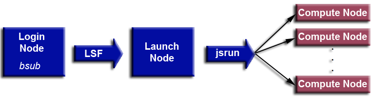
Environment Variables
- By default, LSF will import most (if not all) of your environment variables so they are available to your job.
- If for some reason you are missing environment variables, you can use the #BSUB/bsub -env option to specify variables to import. See the man page for details.
- Additionally, LSF provides a number of its own environment variables. Some of these may be useful for querying purposes within your batch script. The table below lists a few common ones.
| Variable | Description |
|---|---|
| LSB_JOBID | The ID assigned to the job by LSF |
| LSB_JOBNAME | The job's name |
| LS_JOBPID | The job's process ID |
| LSB_JOBINDEX | The job's index (if it belongs to a job array) |
| LSB_HOSTS | The hosts assigned to run the job |
| LSB_QUEUE | The queue from which the job was dispatched |
| LS_SUBCWD | The directory from which the job was submitted |
- To see the entire list of LSF environment variables, simply use a command like printenv, set or setenv (shell dependent) in your batch script, and look for variables that start with LSB_ or LS_.
Interactive Jobs: bsub and lalloc commands
- Interactive jobs are often useful for quick debugging and testing purposes:
- Allow you to acquire an allocation of compute nodes that can be interacted with from the shell command line.
- No handing things over to LSF, and then waiting for the job to complete.
- Easy to experiment with multiple "on the fly" runs.
- There are two main "flavors" of interactive jobs:
- Pseudo-terminal shell - uses your existing SSH login window
- Xterm - launches a new window using your default login shell
- The LSF bsub command, and the LC lalloc command can both be used for interactive jobs.
- Examples:
Starting a pseudo-terminal interactive job using bsub:
From a login node, the bsub command is used to request 4 nodes in an Interactive pseudo-terminal, X11 Forwarding, Wall clock limit of 10 minutes, in a tcsh shell. After the dispatch the interactive session starts on the first compute node (by default). The bquery -X command is used to display the compute nodes allocated for this job.
rzansel61% bsub -nnodes 4 -Ip -XF -W 10 /bin/tcsh
Job <206798> is submitted to default queue <pdebug>.
<<ssh X11 forwarding job>>
<<Waiting for dispatch ...>>
<<Starting on rzansel62>>

rzansel5% bquery -X
JOBID   USER    STAT  QUEUE      FROM_HOST   EXEC_HOST   JOB_NAME   SUBMIT_TIME
206798  blaise  RUN   pdebug     rzansel61   1*rzansel62 /bin/tcsh  Aug 28 11:53
                                             40*rzansel5
                                             40*rzansel6
                                             40*rzansel29
                                             40*rzansel9
Starting a pseudo-terminal interactive job using lalloc:
This same action can be performed more simply using LC's lalloc command. Note that by default, lalloc will use the first compute node as a private launch node. For example:
sierra4362% lalloc 4
+ exec bsub -nnodes 4 -Is -XF -W 60 -core_isolation 2 /usr/tce/packages/lalloc/lalloc-2.0/bin/lexec
Job <281904> is submitted to default queue <pbatch>.
<<ssh X11 forwarding job>>
<<Waiting for dispatch ...>>
<<Starting on sierra4370>>
<<Waiting for JSM to become ready ...>>
<<Redirecting to compute node sierra1214, setting up as private launch node>>
sierra1214%
Starting an xterm interactive job using bsub:
Similar, but opens a new xterm window on the first compute node instead of a tcsh shell in the existing window.
The xterm options follow the xterm command.
sierra4358% bsub -nnodes 4 -XF xterm -sb -ls -fn ergo17 -rightbar
Job <22530> is submitted to default queue <pbatch>.
<<ssh X11 forwarding job>>
<<Waiting for dispatch ...>>
sierra4358%
[ xterm running on first compute node appears on screen at this point ]
Starting an xterm interactive job using lalloc:
Same as previous bsub xterm example, but using lalloc
rzansel61% lalloc 4 xterm
+ exec bsub -nnodes 4 -Is -XF -W 60 -core_isolation 2 /usr/tce/packages/lalloc/lalloc-2.0/bin/lexec xterm
Job <219502> is submitted to default queue <pdebug>.
<<ssh X11 forwarding job>>
<<Waiting for dispatch ...>>
<<Starting on rzansel62>>
<<Waiting for JSM to become ready ...>>
<<Redirecting to compute node rzansel1, setting up as private launch node>>
[ xterm running on first compute node appears on screen at this point ]- How it works:
- Issuing the bsub command from a login node results in control being dispatched to a launch node.
- An allocation of compute nodes is acquired. If not specified, the default is one node.
- The compute node allocation will be in the default queue, usually pbatch. The desired queue can be explicitly specified with the bsub -q or lalloc -q option.
- When ready, your pseudo-terminal or xterm session will run on the first compute node (default at LC). From there, you can use the jsrun command to launch parallel tasks on the compute nodes.
- Usage notes:
- Most of the other bjob options not shown should work as expected.
- For lalloc usage, simple type: lalloc
- Exiting the pseudo-terminal shell, or the xterm, will terminate the job.
Launching Jobs: the lrun command
- The lrun command was developed by LC to make job launching syntax easier for most types of jobs. It can be used as an alternative to the jsrun command (discussed next).
- Like the jsrun command, its purpose is similar to srun/mpirun used on other LC clusters, but its syntax is different.
- Basic syntax (described in detail below):
lrun [lrun_options] [jsrun_options(subset)] [executable] [executable_args] - lrun options are shown in the table below. Note that the same usage information can be found by simply typing lrun when you are logged in.
- Notes:
- LC also provides an srun wrapper for the lrun command for compatibility with the srun command used on other LC systems.
- A discussion on which job launch command should be used can be found in the Quickstart Guide section 12.
| Common Options | Description |
|---|---|
| -N | Number of nodes within the allocation to use. If used, either the -T or -n option must also be used. |
| -T | Number of tasks per node. If -N is not specified, all nodes in the allocation are used. |
| -n -p |
Number of tasks. If -N is not specified, all nodes in the allocation are used. Tasks are evenly spaced over the number of nodes used. |
| -1 | Used for building on a compute node instead of a launch node. For example: lrun -1 make Uses only 1 task on 1 node of the allocation. |
| -M "-gpu" | Turns on CUDA-aware Spectrum MPI |
| Other Options | --adv_map Improved mapping but simultaneous runs may be serialized --threads=<nthreads> Sets env var OMP_NUM_THREADS to nthreads --smt=<1|2|3|4> Set smt level (default 1), OMP_NUM_THREADS overrides --pack Pack nodes with job steps (defaults to -c 1 -g 0) --mpibind=on Force use mpibind in --pack class="fixed-light" mode instead of jsrun's bind -c <ncores_per_task> Required COREs per MPI task (--pack uses for placement) -g <ngpus_per_task> Required GPUs per MPI task (--pack uses for placement) -W <time_limit> Sends SIGTERM to jsrun after minutes or H:M or H:M:S --bind=off No binding/mpibind used in default or --pack mode --mpibind=off Do not use mpibind (disables binding in default mode) --gpubind=off Mpibind binds only cores (CUDA_VISIBLE_DEVICES unset) --core=<format> Sets both CPU & GPU coredump env vars to <format> --core_delay=<secs> Set LLNL_COREDUMP_WAIT_FOR_OTHERS to <secs> --core_cpu=<format> Sets LLNL_COREDUMP_FORMAT_CPU to <format> --core_gpu=<format> Sets LLNL_COREDUMP_FORMAT_GPU to <format> where <format> may be core|lwcore|none|core=<mpirank>|lwcore=<mpirank> -X <0|1> Sets --exit_on_error to 0|1 (default 1) -v Verbose mode, show jsrun command and any set env vars -vvv Makes jsrun wrapper verbose also (core dump settings) |
| Additional Information | JSRUN OPTIONS INCOMPATIBLE WITH LRUN (others should be compatible): -a, -r, -m, -l, -K, -d, -J (and long versions like --tasks_per_rs, --nrs) Note: -n, -c, -g redefined to have different behavior than jsrun's version. ENVIRONMENT VARIABLES THAT LRUN/MPIBIND LOOKS AT IF SET: MPIBIND_EXE <path> Sets mpibind used by lrun, defaults to: /usr/tce/packages/lrun/lrun-2019.05.07/bin/mpibind10 OMP_NUM_THREADS # If not set, mpibind maximizes based on smt and cores OMP_PROC_BIND <mode> Defaults to 'spread' unless set to 'close' or 'master' MPIBIND <j|jj|jjj> Sets verbosity level, more j's -> more output Spaces are optional in single character options (i.e., -T4 or -T 4 valid) Example invocation: lrun -T4 js_task_info |
- Examples - assuming that the total node allocation is 8 nodes (bsub -nnodes 8):
| lrun -N6 -T16 a.out | Launches 16 tasks on each of 6 nodes = 96 tasks |
| lrun -n128 a.out | Launches 128 tasks evenly over 8 nodes |
| lrun -T16 a.out | Launches 16 tasks one each of 8 nodes = 128 tasks |
| lrun -1 make | Launches 1 make process on 1 node |
Launching jobs: the jsrun Command and Resource Sets
- The jsrun command is the IBM provided parallel job launch command for Sierra systems.
- Replaces srun and mpirun used on other LC systems:
- Similar in function, but very different conceptually and in syntax.
- Based upon an abstraction called resource sets.
- Basic syntax (described in detail below):
jsrun [options] [executable] - Developed by IBM for the LLNL and Oak Ridge CORAL systems:
- Part of the IBM Job Step Manager (JSM) software package for managing a job allocation provided by the resource manager.
- Integrated into the IBM Spectrum LSF Workload Manager.
- A discussion on which job launch command should be used can be found in the Quickstart Guide section 12.
Resource Sets
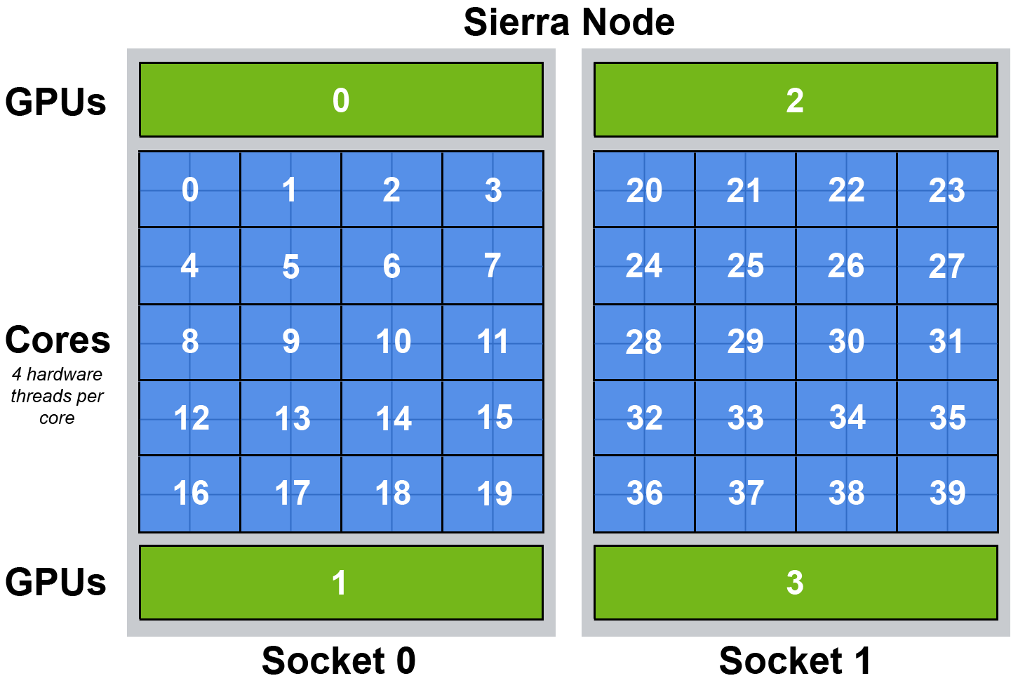
- A Sierra node consists of the following resources per node - see diagram at right:
- 40 cores; 20 per socket; Note Two cores on each socket are reserved for the operating system, and are therefore not included.
- 160 hardware threads; 4 per core
- 4 GPUs; 2 per socket
- In the simplest sense, a resource set describes how a node's resources should look to a job.
- A basic resource set definition consists of:
- Number of tasks
- Number of cores
- Number of GPUs
- Memory allocation
- Rules:
- Described in terms of a single node's resources
- Can span sockets on a node
- Cannot span multiple nodes
- Defaults are used if any resource is not explicitly specified.
- Example Resource Sets:
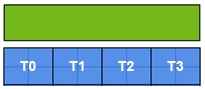
Fits on 1 socket
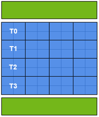
Fits on 1 socket
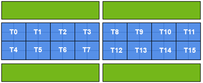
Requires both sockets
-
After defining the resource set, you need to define:
- The number of Nodes required for the job
- How many Resource Sets should be on each node
- The total number of Resource Sets for the entire job
- These parameters are then provided to the jsrun command as options/flags.
- Examples with jsrun options shown:
4 tasks ♦ 4 Cores ♦ 1 GPU
-a4 -c4 -g1
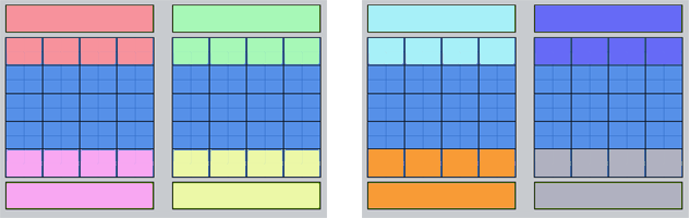
4 resource sets per node ♦ 8 resource sets total
-r4 -n8
4 Tasks ♦ 16 Cores ♦ 2 GPUs
-a4 -c16 -g2
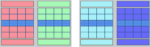
2 resource sets per node ♦ 4 resource sets total
-r4 -n4
jsrun Options
- The table below describes a number of commonly used jsrun options. See the jsrun man page for details.
- Additionally, a very good, and detailed presentation on the jsrun command is available at: https://www.olcf.ornl.gov/wp-content/uploads/2018/02/SummitJobLaunch.pdf.
| Option (short) | Option (long) | Description |
|---|---|---|
| -a | --tasks_per_rs | Number of tasks per resource set |
| -b | --bind | Specifies the binding of tasks within a resource set. Can be none, rs (resource set), or packed:smt#. See the jsrun man page for details. |
| -c | --cpu_per_rs | Number of CPUs (cores) per resource set. |
| -d | --launch_distribution | Specifies how task are started on resource sets. Options are cyclic, packed, plane:#. See the man page for details. |
| -E -F -D |
--env var --env_eval --env_no_propagate |
Specify how to handle environment variables. See the man page for details. |
| -g | --gpu_per_rs | Number of GPUs per resource set |
| -l | --latency priority | Latency Priority. Controls layout priorities. Can currently be cpu-cpu, gpu-cpu, gpu-gpu, memory-memory, cpu-memory or gpu-memory. See the man page for details. |
| -n | --nrs | Total number of resource sets for the job. |
| -M "-gpu" | --smpiargs "-gpu" | Turns on CUDA-aware Spectrum MPI |
| -m | --memory_per_rs | Specifies the number of megabytes of memory (1,048,756 bytes) to assign to a resource set. Use the -S option to view the memory setting. |
| -p | --np | Number of tasks to start. By default, each task is assigned its own resource set that contains a single CPU. |
| -r | --rs_per_host | Number of resource sets per host (node) |
| -S filename | --save_resources | Specifies that the resources used for the job step are written to filename. |
| -t -o -e -k |
--stdio_input --stdio_stdout --stdio_mode --stdio_stderr |
Specifies how to handle stdio, stdout and stderr. See the man page for details. |
| -V | --version | Displays the version of jsrun Job Step Manager (JSM). |
- Examples:
These examples assume that 40 cores per node are available for user tasks (4 are reserved for the operating system), and each node has 4 GPUs.
White space between an option and its argument is optional.
| jsrun Command | Description | Diagram |
|---|---|---|
| jsrun -p72 a.out | 72 tasks, no GPUs 2 nodes, 40 tasks on node1, 32 tasks on node2 |
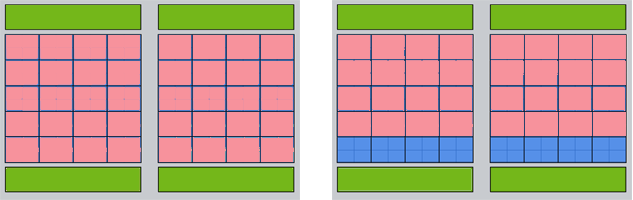
|
| jsrun -n8 -a1 -c1 -g1 a.out | 8 resource sets, each with 1 task and 1 GPU 2 nodes, 2 tasks per socket |

|
| jsrun -n8 -a1 -c4 -g1 -bpacked:4 a.out | 8 resource sets each with 1 task with 4 threads (cores) and 1 GPU 2 nodes, 2 tasks per socket |
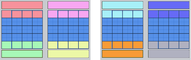
|
| jsrun -n8 -a2 -c2 -g1 a.out | 8 resource sets each with 2 tasks and 1 GPU 2 nodes, 4 tasks per socket |
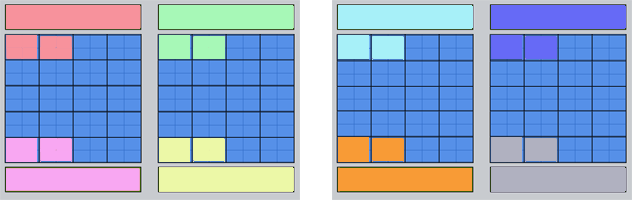
|
| jsrun -n4 -a1 -c1 -g2 a.out | 4 resource sets each with 1 task and 2 GPUs 2 nodes: 1 task per socket |
|
Job Dependencies
#BSUB -w Option
- As with other batch systems, LSF provides a way to place dependencies on jobs to prevent them from running until other jobs have started, completed, etc.
- The #BSUB -w option is used to accomplish this. The syntax is:
#BSUB -w dependency_expression - A dependency expression is a logical expression comprised of one or more dependency conditions. It can include relational operators such as:
&& (AND) || (OR) ! (NOT)
> >= <
<= == !=
- Several dependency examples are shown in the table below:
| Example | Description |
|---|---|
| #BSUB -w started(22345) | Job will not start until job 22345 starts. Job 22345 is considered to have started if is in any of the following states: USUSP, SSUSP, DONE, EXIT or RUN (with any pre-execution command specified by bsub -E completed) |
| #BSUB -w done(22345) #BSUB -w 22345 |
Job will not start until job 22345 has a state of DONE (completed normally). If a job ID is given with no condition, done() is assumed. |
| #BSUB -w exit(22345) | Job will not start until job 22345 has a state of EXIT (completed abnormally) |
| #BSUB -w ended(22345) | Job will not start until job 22345 has a state of EXIT or DONE |
| #BSUB -w done(22345) && started(33445) | Job will not start until job 22345 has a state of DONE and job 33445 has started |
- Usage notes:
- The -w option can be used with the bsub command, but it is extremely limited because parens and relational operators cannot be included with the command.
- LSF requires that valid jobids be specified - can't use non-existent jobids.
- To remove dependencies for a job, use the command: bmod -wn jobid
bjdepinfo Command
- The bjdepinfo command can be used to view job dependency information. More useful than the bquery -l command.
- See the bjdepinfo man page and/or the LSF Documentation for details.
- Examples are shown below:
    % bjdepinfo 30290
    JOBID          PARENT         PARENT_STATUS  PARENT_NAME  LEVEL
    30290          30285          RUN            *mmat 500    1


    % bjdepinfo -r3 30290
    JOBID          PARENT         PARENT_STATUS  PARENT_NAME  LEVEL
    30290          30285          RUN            *mmat 500    1
    30285          30271          DONE           *mmat 500    2
    30271          30267          DONE           *mmat 500    3
Monitoring Jobs: lsfjobs, bquery bpeek, bhist commands
LSF provides several commands for monitoring jobs. Additionally LC provides a locally developed command for monitoring jobs called lsfjobs.
lsfjobs
- LC's lsfjobs command is useful for displaying a summary of queued and running jobs, along with a summary of each queue's usage.
- Usage information - use any of the commands: lsfjobs -h, lsfjobs -help, lsfjobs -man
- Various options are available for filtering output by user, group, jobid, queue, job state, completion time, etc.
- Output can be easily customized and include additional fields of information. Job states are described - over 20 different states possible.
- Example output below:
**********************************
* Host:    - lassen - lassen708  *
* Date:    - 08/26/2019 14:38:34 *
* Cmd:     - lsfjobs             *
**********************************

*********************************************************************************************************************************
* JOBID    SLOTS    PTILE    HOSTS    USER            STATE            PRIO        QUEUE        GROUP    REMAINING        LIMIT *
*********************************************************************************************************************************
  486957       80       40        2    liii3             RUN               -       pdebug      smt4lnn        04:00      2:00:00
  486509      640       40       16    joqqm             RUN               -      standby     hohlfoam        12:00      2:00:00
  487107     1600       40       40    mnss3             RUN               -      pbatch0      wbronze        17:00      1:00:00
  487176     1280       40       32    dirrr211          RUN               -      pbatch0     stanford        25:00      0:40:00
  486908       40       40        1    samuu4            RUN               -      pbatch3        dbalf     11:51:00     12:00:00
  ....
  486910       40       40        1    samuu4            RUN               -      pbatch3        dbalf     11:51:00     12:00:00
  487054       40       40        1    samuu4            RUN               -      pbatch3        dbalf     11:51:00     12:00:00
  -----------------------------------------------------------
  477171    10240       40      256    miss6666       TOOFEW         1413.00      pbatch0      cbronze            -     12:00:00
  -----------------------------------------------------------
  487173      160       40        4    land3211    SLOTLIMIT          600.50      pbatch2         vfib            -      2:00:00
  486770      320       40        8    tamgg4      SLOTLIMIT          200.80      pbatch3     nonadiab            -     12:00:00
  487222       40       40        1    samww2      SLOTLIMIT          200.50      pbatch3        dbalf            -     12:00:00
  -----------------------------------------------------------
  486171       40       40        1    munddd33       DEPEND          200.50      pbatch3      feedopt            -     12:00:00
  487013      640       40       16    joww2          DEPEND           40.50      standby     hohlfoam            -      2:00:00
  -----------------------------------------------------------
  394147      640       40       16    ecqq2344         HELD          401.20       pbatch     exalearn            -      9:00:00
  394162      640       40       16    ecqq2344         HELD          401.10       pbatch     exalearn            -      9:00:00

***************************************************************
* HOST_GROUP       TOTAL   DOWN    RSVD/BUSY   FREE   HOSTS   *
***************************************************************
   batch_hosts        752     15          737      0   lassen[37-680,720-827]
   debug_hosts         36      0           22     14   lassen[1-36]

*****************************************************************************************************
* QUEUE          TOTAL  DOWN   RSVD/BUSY   FREE   DEFAULTTIME      MAXTIME  STATE     HOST_GROUP(S) *
*****************************************************************************************************
   exempt           752    15         737      0          None    Unlimited  Active    batch_hosts
   expedite         752    15         737      0          None    Unlimited  Active    batch_hosts
   pall             788    15         759     14          None    Unlimited  Active    batch_hosts,debug_hosts
   pbatch           752    15         737      0         30:00     12:00:00  Active    batch_hosts
   pbatch0          752    15         737      0         30:00     12:00:00  Active    batch_hosts
   pbatch1          752    15         737      0         30:00     12:00:00  Active    batch_hosts
   pbatch2          752    15         737      0         30:00     12:00:00  Active    batch_hosts
   pbatch3          752    15         737      0         30:00     12:00:00  Active    batch_hosts
   pdebug            36     0          22     14         30:00      2:00:00  Active    debug_hosts
   standby          788    15         759     14          None    Unlimited  Active    batch_hosts,debug_hosts
bquery
- Provides a number of options for displaying a range of job information - from summary to detailed.
- The table below shows some of the more commonly used options.
- See the bquery man page and/or the LSF Documentation for details.
| Command | Description | Example |
|---|---|---|
| bquery | Show your currently queued and running jobs | |
| bquery -u all | Show queued and running jobs for all users | |
| bquery -a | Show jobs in all states including recently completed | |
| bquery -d | Show only recently completed jobs | |
| bquery -l bquery -l 22334 bquery -l -u all |
Show long listing of detailed job information Show long listing for job 22334 Show long listing for all user jobs |
|
| bquery -o [format string] | Specifies options for customized format bquery output. See the documentation for details. | |
| bquery -p bquery -p -u all |
Show pending jobs and reason why Show pending jobs for all users |
|
| bquery -r bquery -r -u all |
Show running jobs Show running jobs for all users |
|
| bquery -X | Show host names (uncondensed) |
bpeek
- Allows you to view stdout/stderr of currently running jobs.
- Provides several options for selecting jobs by queue, name, jobid.
- See the bpeek man page and/or LSF documentation for details.
- Examples below:
| Command | Description |
|---|---|
| bpeek 27239 | Show output from jobid 27239 |
| bpeek -J myjob | Show output for most recent job named "myjob" |
| bpeek -f | Shows output of most recent job by looping with the command tail -f. When the job is done, the bpeek command exits. |
| bpeek -q | Displays output of the most recent job in the specified queue. |
bhist
- By default, displays information about your pending, running, and suspended jobs.
- Also provides options for displaying information about recently completed jobs, and for filtering output by job name, queue, user, group, start-end times, and more.
- See the bhist man page and/or LSF documentation for details.
- Example below - shows running, queued and recently completed jobs:
% bhist -a
    Summary of time in seconds spent in various states:
    JOBID   USER    JOB_NAME  PEND    PSUSP   RUN     USUSP   SSUSP   UNKWN   TOTAL
    27227   user22  run.245   2       0       204     0       0       0       206
    27228   user22  run.247   2       0       294     0       0       0       296
    27239   user22  runtest   4       0       344     0       0       0       348
    27240   user22  run.248   2       0       314     0       0       0       316
    27241   user22  runtest   1       0       313     0       0       0       314
    27243   user22  run.249   13      0       1532    0       0       0       1545
    27244   user22  run.255   0       0       186     0       0       0       186
    27245   user22  run.267   1       0       15      0       0       0       16
    27246   user22  run.288   2       0       12      0       0       0       14
Job States
- LSF job monitoring commands display a job's state. The most commonly seen ones are shown in the table below.
| State | Description |
|---|---|
| DONE | Job completed normally |
| EXIT | Job completed abnormally |
| PEND | Job is pending, queued |
| PSUSP | Job was suspended (either by the user or an administrator) while pending |
| RUN | Job is running |
| SSUSP | Job was suspended by the system after starting |
| USUSP | Job was suspended (either by the user or an administrator) after starting |
Suspending / Resuming Jobs: bstop, bresume commands
bstop and bresume Commands
- LSF provides support for user-level suspension and resumption of running and queued jobs.
- However, at LC, the bstop command is used to suspend queued jobs only. Note This is different from the LSF default behavior and documentation, which allows suspension of running jobs.
- Queued jobs that have been suspended will show a PSUSP state
- The bresume command is used to resume suspended jobs.
- Jobs can be specified by jobid, host, job name, group, queue and other criteria. In the examples below, jobid is used.
- See the bstop man page, bresume man page and/or LSF documentation for details.
- Examples below:
Suspend a queued job, and then resume
    % bquery
    JOBID   USER    STAT  QUEUE      FROM_HOST   EXEC_HOST   JOB_NAME   SUBMIT_TIME
    31411   user22  PEND  pdebug     sierra4360              bmbtest    Apr 13 12:11

    % bstop 31411
    Job <31411> is being stopped

    % bquery
    JOBID   USER    STAT  QUEUE      FROM_HOST   EXEC_HOST   JOB_NAME   SUBMIT_TIME
    31411   user22  PSUSP pdebug     sierra4360              bmbtest    Apr 13 12:11

    % bresume 31411
    Job <31411> is being resumed

    % bquery
    bquery
    JOBID   USER    STAT  QUEUE      FROM_HOST   EXEC_HOST   JOB_NAME   SUBMIT_TIME
    31411   user22  RUN   pdebug     sierra4360  1*launch_ho bmbtest    Apr 13 12:11
                                                 400*debug_hosts
Modifying Jobs: bmod command
bmod Command
- The bmod command is used to modify the options of a previously submitted job.
- Simply use the desired bsub option with bmod, providing a new value. For example, to modify the wallclock time for jobid 22345:
bmod -W 500 22345>
- You can modify all options for a pending job, even if the corresponding bsub command option was not specified. This comes in handy in case you forgot an option when the job was originally submitted.
- You can also "reset" options to their original or default values by appending a lowercase n to the desired option (no whitespace). For example to reset the queue to the original submission value:
bmod -qn 22345 - For running jobs, there are very few, if any, useful options that can be changed.
- See the bmod man page and/or LSF documentation for details.
- The bhist -l command can be used to view a history of which job parameters have been changed - they appear near the end of the output. For example:
% bhist -l 31788

    ...[previous output omitted]

    Fri Apr 13 14:10:20: Parameters of Job are changed:
        Output file change to : /g/g0/user22/lsf/
        User group changes to: guests
        run limit changes to : 55.0 minutes;
    Fri Apr 13 14:13:40: Parameters of Job are changed:
        Job queue changes to : pbatch
        Output file change to : /g/g0/user22/lsf/
        User group changes to: guests;
    Fri Apr 13 14:30:08: Parameters of Job are changed:
        Job queue changes to : standby
        Output file change to : /g/g0/user22/lsf/
        User group changes to: guests;

    ...[following output omitted]
Signaling / Killing Jobs: bkill command
bkill Command
- The bkill command is used to both terminate jobs and to send signals to jobs.
- Similar to the kill command found in Unix/Linux operating systems - can be used to send various signals (not just SIGTERM and SIGKILL) to jobs.
- Can accept both numbers and names for signals.
- In additional to jobid, jobs can be identified by queue, host, group, job name, user, and more.
- For a list of accepted signal names, run bkill -l
- See the bkill man page and/or LSF documentation for details.
For general details on Linux signals see http://man7.org/linux/man-pages/man7/signal.7.html. - Examples:
| Command | Description |
|---|---|
| bkill 22345 bkill 34455 24455 |
Force a job(s) to stop by sending SIGINT, SIGTERM, and SIGKILL. These signals are sent in that order, so users can write applications such that they will trap SIGINT and/or SIGTERM and exit in a controlled manner. |
| bkill -s HUP 22345 | Send SIGHUP to job 22345. Note When specifying a signal by name, omit SIG from the name. |
| bkill -s 9 22345 | Send signal 9 to job 22345 |
| bkill -s STOP -q pdebug | Send a SIGSTOP signal to the most recent job in the pdebug queue |
CUDA-aware MPI
- CUDA-aware MPI allows GPU buffers (allocated with cudaMalloc) to be used directly in MPI calls. Without CUDA-Aware MPI data must be copied manually to/from a CPU buffer (using cudaMemcpy) before/after passing data in MPI calls. For example:
| Without CUDA-aware MPI - need to copy data between GPU and CPU memory before/after MPI send/receive operations. | With CUDA-aware MPI - data is transferred directly to/from GPU memory by MPI send/receive operations. |
|---|---|
//MPI rank 0 cudaMemcpy(sendbuf_h,sendbuf_d,size,cudaMemcpyDeviceToHost); MPI_Send(sendbuf_h,size,MPI_CHAR,1,tag,MPI_COMM_WORLD); //MPI rank 1 MPI_Recv(recbuf_h,size,MPI_CHAR,0,tag,MPI_COMM_WORLD, &status); cudaMemcpy(recbuf_d,recbuf_h,size,cudaMemcpyHostToDevice); |
//MPI rank 0 MPI_Send(sendbuf_d,size,MPI_CHAR,1,tag,MPI_COMM_WORLD); //MPI rank 1 MPI_Recv(recbuf_d,size,MPI_CHAR,0,tag,MPI_COMM_WORLD, &status); |
- IBM Spectrum MPI on CORAL systems is CUDA-aware. However, users are required to "turn on" this feature using a run-time flag with lrun or jsrun. For example:
lrun -M "-gpu"
jsrun -M "-gpu" - Caveat Do NOT use the MPIX_Query_cuda_support() routine or the preprocessor constant MPIX_CUDA_AWARE_SUPPORT to determine if Spectrum MPI is CUDA-aware. This routine has either been removed from the IBM implementation, or will always return false (older versions).
- Additional Information:
- An Introduction to CUDA-Aware MPI: https://devblogs.nvidia.com/introduction-cuda-aware-mpi/
- MPI Status Updates and Performance Suggestions: 2019.05.09.MPI_UpdatesPerformance.Karlin.pdf
Process, Thread and GPU Binding: js_task_info
- Application performance can be significantly impacted by the way MPI tasks and OpenMP threads are bound to cores and GPUs.
- Important The binding behaviors of lrun and jsrun are very different, and not obvious to users. The jsrun command in particular often requires careful consideration in order to obtain optimal bindings.
- The js_task_info utility provides an easy way to see exactly how tasks and threads are being bound. Simply run js_task_info with lrun or jsrun as you would your application.
- The lrun -v flag shows the actual jsrun command that is used "under the hood". The -vvv flag can be used with both lrun and jsrun to see additional details, including environment variables.
- Several examples, using 1 node, are shown below. Note that each thread on an SMT4 core counts as a "cpu" (4*44 cores = 176 cpus) in the output, and that the first 8 "cpus" [0-7] are reserved for core isolation.
% lrun -n4 js_task_info
Task 0 ( 0/4, 0/4 ) is bound to cpu[s] 8,12,16,20,24,28,32,36,40,44 on host lassen2 with OMP_NUM_THREADS=10 and with OMP_PLACES={8},{12},{16},{20},{24},{28},{32},{36},{40},{44} and CUDA_VISIBLE_DEVICES=0
Task 1 ( 1/4, 1/4 ) is bound to cpu[s] 48,52,56,60,64,68,72,76,80,84 on host lassen2 with OMP_NUM_THREADS=10 and with OMP_PLACES={48},{52},{56},{60},{64},{68},{72},{76},{80},{84} and CUDA_VISIBLE_DEVICES=1
Task 3 ( 3/4, 3/4 ) is bound to cpu[s] 136,140,144,148,152,156,160,164,168,172 on host lassen2 with OMP_NUM_THREADS=10 and with OMP_PLACES={136},{140},{144},{148},{152},{156},{160},{164},{168},{172} and CUDA_VISIBLE_DEVICES=3
Task 2 ( 2/4, 2/4 ) is bound to cpu[s] 96,100,104,108,112,116,120,124,128,132 on host lassen2 with OMP_NUM_THREADS=10 and with OMP_PLACES={96},{100},{104},{108},{112},{116},{120},{124},{128},{132} and CUDA_VISIBLE_DEVICES=2

% lrun -n4 --smt=4 -v js_task_info
+ export MPIBIND+=.smt=4
+ exec /usr/tce/packages/jsrun/jsrun-2019.05.02/bin/jsrun --np 4 --nrs 1 -c ALL_CPUS -g ALL_GPUS -d plane:4 -b none -X 1 /usr/tce/packages/lrun/lrun-2019.05.07/bin/mpibind10 js_task_info
Task 0 ( 0/4, 0/4 ) is bound to cpu[s] 8-47 on host lassen2 with OMP_NUM_THREADS=40 and with OMP_PLACES={8},{9},{10},{11},{12},{13},{14},{15},{16},{17},{18},{19},{20},{21},{22},{23},{24},{25},{26},{27},{28},{29},{30},{31},{32},{33},{34},{35},{36},{37},{38},{39},{40},{41},{42},{43},{44},{45},{46},{47} and CUDA_VISIBLE_DEVICES=0
Task 1 ( 1/4, 1/4 ) is bound to cpu[s] 48-87 on host lassen2 with OMP_NUM_THREADS=40 and with OMP_PLACES={48},{49},{50},{51},{52},{53},{54},{55},{56},{57},{58},{59},{60},{61},{62},{63},{64},{65},{66},{67},{68},{69},{70},{71},{72},{73},{74},{75},{76},{77},{78},{79},{80},{81},{82},{83},{84},{85},{86},{87} and CUDA_VISIBLE_DEVICES=1
Task 2 ( 2/4, 2/4 ) is bound to cpu[s] 96-135 on host lassen2 with OMP_NUM_THREADS=40 and with OMP_PLACES={96},{97},{98},{99},{100},{101},{102},{103},{104},{105},{106},{107},{108},{109},{110},{111},{112},{113},{114},{115},{116},{117},{118},{119},{120},{121},{122},{123},{124},{125},{126},{127},{128},{129},{130},{131},{132},{133},{134},{135} and CUDA_VISIBLE_DEVICES=2
Task 3 ( 3/4, 3/4 ) is bound to cpu[s] 136-175 on host lassen2 with OMP_NUM_THREADS=40 and with OMP_PLACES={136},{137},{138},{139},{140},{141},{142},{143},{144},{145},{146},{147},{148},{149},{150},{151},{152},{153},{154},{155},{156},{157},{158},{159},{160},{161},{162},{163},{164},{165},{166},{167},{168},{169},{170},{171},{172},{173},{174},{175} and CUDA_VISIBLE_DEVICES=3

% jsrun -p4 js_task_info
Task 0 ( 0/4, 0/4 ) is bound to cpu[s] 8-11 on host lassen2 with OMP_NUM_THREADS=4 and with OMP_PLACES={8:4}
Task 1 ( 1/4, 1/4 ) is bound to cpu[s] 12-15 on host lassen2 with OMP_NUM_THREADS=4 and with OMP_PLACES={12:4}
Task 2 ( 2/4, 2/4 ) is bound to cpu[s] 16-19 on host lassen2 with OMP_NUM_THREADS=4 and with OMP_PLACES={16:4}
Task 3 ( 3/4, 3/4 ) is bound to cpu[s] 20-23 on host lassen2 with OMP_NUM_THREADS=4 and with OMP_PLACES={20:4}

% jsrun -r4 -c10 -a1 -g1 js_task_info
Task 0 ( 0/4, 0/4 ) is bound to cpu[s] 8-11 on host lassen2 with OMP_NUM_THREADS=4 and with OMP_PLACES={8:4} and CUDA_VISIBLE_DEVICES=0
Task 1 ( 1/4, 1/4 ) is bound to cpu[s] 48-51 on host lassen2 with OMP_NUM_THREADS=4 and with OMP_PLACES={48:4} and CUDA_VISIBLE_DEVICES=1
Task 2 ( 2/4, 2/4 ) is bound to cpu[s] 96-99 on host lassen2 with OMP_NUM_THREADS=4 and with OMP_PLACES={96:4} and CUDA_VISIBLE_DEVICES=2
Task 3 ( 3/4, 3/4 ) is bound to cpu[s] 136-139 on host lassen2 with OMP_NUM_THREADS=4 and with OMP_PLACES={136:4} and CUDA_VISIBLE_DEVICES=3

% jsrun -r4 -c10 -a1 -g1 -b rs js_task_info
Task 0 ( 0/4, 0/4 ) is bound to cpu[s] 8-47 on host lassen2 with OMP_NUM_THREADS=40 and with OMP_PLACES={8:4},{12:4},{16:4},{20:4},{24:4},{28:4},{32:4},{36:4},{40:4},{44:4} and CUDA_VISIBLE_DEVICES=0
Task 1 ( 1/4, 1/4 ) is bound to cpu[s] 48-87 on host lassen2 with OMP_NUM_THREADS=40 and with OMP_PLACES={48:4},{52:4},{56:4},{60:4},{64:4},{68:4},{72:4},{76:4},{80:4},{84:4} and CUDA_VISIBLE_DEVICES=1
Task 2 ( 2/4, 2/4 ) is bound to cpu[s] 96-135 on host lassen2 with OMP_NUM_THREADS=40 and with OMP_PLACES={96:4},{100:4},{104:4},{108:4},{112:4},{116:4},{120:4},{124:4},{128:4},{132:4} and CUDA_VISIBLE_DEVICES=2
Task 3 ( 3/4, 3/4 ) is bound to cpu[s] 136-175 on host lassen2 with OMP_NUM_THREADS=40 and with OMP_PLACES={136:4},{140:4},{144:4},{148:4},{152:4},{156:4},{160:4},{164:4},{168:4},{172:4} and CUDA_VISIBLE_DEVICES=3
Node Diagnostics: check_sierra_nodes
- This LC utility allows you to check for bad nodes within your allocation before launching your actual job. For example:
sierra4368% check_sierra_nodes
STARTED: 'jsrun -r 1 -g 4 test_sierra_node -mpi -q' at Thu Aug 23 15:48:14 PDT 2018
SUCCESS: Returned 0 (all, including MPI, tests passed) at Thu Aug 23 15:48:22 PDT 2018
- The last line will start with SUCCESS if no bad nodes were found and the return code will be 0.
- Failure messages should be reported to the LC Hotline.
- Note This diagnostic and other detailed "health checks" are run after every batch allocation, so routine use of this test has been deprecated. For additional details, see the discussion in the Quickstart Guide.
Burst Buffer Usage
- A burst buffer is a fast and intermediate storage layer positioned between the front-end computing processes and the back-end storage systems.
- The goal of a burst buffer is to improve application I/O performance and reduce pressure on the parallel file system.
- Example use: applications that write checkpoints; faster than writing to disk; computation can resume more quickly while burst buffer data is asynchronously moved to disk.
- For Sierra systems, and the Ray Early Access system, the burst buffer is implemented as a 1.6 TB SSD (Solid State Drive) storage device local to each compute node. This drive takes advantage of NVMe over fabrics technologies, which allows remote access to the data without causing interference to an application running on the compute node itself.
- Sierra's burst buffer hardware is covered in the NVMe PCIe SSD (Burst Buffer) section of this tutorial.
- The node-local burst buffer space on sierra, lassen and rzansel compute nodes is managed by the LSF scheduler:
- Users may request a portion of this space for use by a job.
- Once a job is running, the burst buffer space appears as a file system mounted under $BBPATH.
- Users can then access $BBPATH as any other mounted file system.
- Users may also stage-in and stage-out files to/from burst buffer storage.
- In addition, a shared-namespace filesystem (called BSCFS) can be spun up across the disparate storage devices. This allows users to write a shared file across the node-local storage devices.
- On the ray Early Access system, the node-local SSD is simply mounted as /l/nvme on the compute nodes, and is not managed by LSF. It can be used as any other node-local file system for working with files. Additional information for using the burst buffer on ray can be found at: https://lc.llnl.gov/confluence/display/CORALEA/Ray+Burst+Buffers+and+dbcast (internal wiki).
Requesting Burst Buffer Storage for a Job
- Applies to sierra, lassen and rzansel, not ray
- Simply add the -stage storage=#gigabytes flag to your bsub or lalloc command. Some examples are shown below:
bsub -nnodes 4 -stage storage=64 -Is bash Requests 4 nodes with 64 GB storage each, interactive bash shell
lalloc 4 -stage storage=64 Equivalent using lalloc
bsub -stage storage=64 < jobscript Requests 64 GB storage per node using a batch script
- For LSF batch scripts, you can use the #BSUB -stage storage=64 syntax in your script instead of on the bsub command line.
- Allocating burst buffer space typically requires additional time for bsub/lalloc.
- Note As of Sep 2019, the maximum amount of storage that can be requested is 1200 GB (subject to change). Requesting more than this will cause jobs to hang in the queue. In the future, LC plans to implement immediate rejection of a job if it requests storage above the limit.
Using the Burst Buffer Storage Space
- Applies to sierra, lassen, rzansel, not ray
- Once LSF has allocated the nodes for your job, the node-local storage space can be accessed as any other mounted file system.
- For convenience, the path to your node-local storage is set as the $BBPATH environment variable.
- You can cd, cp, ls, rm, mv, vi, etc. files in $BBPATH as normal for other file systems.
- Your programs can conduct I/O to files in $BBPATH as well.
-
Example:
% lalloc 1 -qpdebug -stage storage=64
+ exec bsub -nnodes 1 -qpdebug -stage storage=64 -Is -XF -W 60 -core_isolation 2 /usr/tce/packages/lalloc/lalloc-2.0/bin/lexec
Job <517170> is submitted to queue <pdebug>.
<<ssh X11 forwarding job>>
<<Waiting for dispatch ...>>
<<Starting on lassen710>>
<<Waiting for JSM to become ready ...>>
<<Redirecting to compute node lassen21, setting up as private launch node>>
% echo $BBPATH
/mnt/bb_1d2e8a9f19a8c5dedd3dd9a373b70cc9
% df -h $BBPATH
Filesystem            Size  Used Avail Use% Mounted on
/dev/mapper/bb-bb_35   64G  516M   64G   1% /mnt/bb_1d2e8a9f19a8c5dedd3dd9a373b70cc9
% touch $BBPATH/testfile
% cd $BBPATH
% pwd
/mnt/bb_1d2e8a9f19a8c5dedd3dd9a373b70cc9
% ls -l
total 0
-rw------- 1 user22 user22 0 Sep  6 15:00 testfile
-
For parallel jobs, each task sees the burst buffer mounted as $BBPATH local to its node. A simple parallel usage example using 1 task on each of 2 nodes is shown below.
% cat testscript
#!/bin/tcsh
setenv myrank $OMPI_COMM_WORLD_RANK
setenv node `hostname`
echo "Rank $myrank using burst buffer $BBPATH on $node"
echo "Rank $myrank copying input file to burst buffer"
cp $cwd/input.$myrank  $BBPATH/
echo "Rank $myrank doing work..."
cat $BBPATH/input.$myrank > $BBPATH/output.$myrank
echo -n "Rank $myrank burst buffer shows: "
ls -l $BBPATH
echo "Rank $myrank copying output file to GPFS"
cp $BBPATH/output.$myrank /p/gpfs1/$USER/output/
echo "Rank $myrank done."

% lrun -n2 testscript
Rank 0 using burst buffer /mnt/bb_811dfc9bc5a6896a2cbea4f5f8087212 on rzansel3
Rank 0 copying input file to burst buffer
Rank 0 doing work...
Rank 0 burst buffer shows: total 128
-rw------- 1 user22 user22 170 Sep 10 12:49 input.0
-rw------- 1 user22 user22 170 Sep 10 12:49 output.0
Rank 0 copying output file to GPFS
Rank 0 done.
Rank 1 using burst buffer /mnt/bb_811dfc9bc5a6896a2cbea4f5f8087212 on rzansel5
Rank 1 copying input file to burst buffer
Rank 1 doing work...
Rank 1 burst buffer shows: total 128
-rw------- 1 user22 user22 76 Sep 10 12:49 input.1
-rw------- 1 user22 user22 76 Sep 10 12:49 output.1
Rank 1 copying output file to GPFS
Rank 1 done.

% ls -l /p/gpfs1/user22/output
total 2
-rw------- 1 user22 user22 170 Sep  6 15:53 output.0
-rw------- 1 user22 user22  76 Sep  6 15:53 output.1
Staging Data to/from Burst Buffer Storage
- LSF can automatically move a job's data files in-to and out-of the node-local storage devices. This is achieved through the integration of LSF with IBM's burst buffer software. The two options are:
- bbcmd command line tool, typically employed in user scripts.
- BBAPI C-library API consisting of subroutines called from user source code.
- There are 4 possible "phases" of data movement relating to a single job allocation:
- Stage-in or pre-stage of data: Before an application begins on the compute resources, files are moved from the parallel file system into the burst buffer. The file movement is triggered by a user script with bbcmd commands which has been registered with LSF.
- Data movement during the compute allocation: While the application is running, asynchronous data movement can take place between the burst buffer and parallel file system. This movement can be initiated via the C-library routines or via the command line tool.
- Stage-out or post-stage of data: After the application has completed using the compute resources (but before the burst buffer has been de-allocated), files are moved from the burst buffer to the parallel file system. The file movement is triggered by a user script with bbcmd commands which has been registered with LSF.
- Post-stage finalization: After the stage-out of files has completed, a user script may be called. This allows users to perform book-keeping actions after the data-movement portion of their job has completed. This is done through a user supplied script which is registered with LSF.
- Example workflow using the bbcmd interface:
- Create a stage-in script with bbcmd commands for moving data from the parallel file system to the burst buffer. Make it executable. Also create a corresponding text file that lists the files to be transferred.
- Create stage-out script with bbcmd commands for moving data from the burst buffer to the parallel file system. Make it executable. Also create a corresponding text file that lists the files to be transferred.
- Create a post-stage script and make it executable.
- Create an LSF job script as usual
- Register your stage-in/stage-out scripts with LSF: This is done by submitting your LSF job script with bsub using the -stage <sub-arguments> flag. The sub-arguments are separated by colons, and can include:
- storage=#gigabytes
- in=path-to-stage-in-script
- out=path-to-stage-out-script1, path-to-stage-out-script2
- Alternatively, you can specify the -stage <sub-arguments> flag in your LSF job script using the #BSUB syntax.
- Example: requests 256 GB of storage; stage-in.sh is the user stage-in script, stage-out1.sh is the user stage-out script, stage-out2.sh is the user post-stage finalization script.
bsub -stage "storage=256:in=/p/gpfs1/user22/stage-in.sh:out=/p/gpfs1/user22/stage-out1.sh,/p/gpfs1/user22/stage-out2.sh"
- Notes for stage-out, post-stage scripts: The out=path-to-stage-out-script1,path-to-stage-out-script2 option specifies 2 separate user-created stage-out scripts separated by a comma. The first script is run after the compute allocation has completed, but while the data on the burst buffer may still be accessed. The second script is run after the burst buffer has been de-allocated. If a stage-out1 script is not needed, the argument syntax would be out=,path-to-stage-out-script2. The full path to the scripts should be specified and the scripts must be marked as executable.
- Stage-in / stage-out scripts and file lists: examples coming soon
BBAPI C-library API
- This IBM provided, C-library API provides routines for using Sierra systems burst buffers.
- Requires modification of source code.
- More information can be found at: https://lc.llnl.gov/confluence/display/SIERRA/API+Documentation (internal wiki)
BSCFS:
- This IBM provided, C-library API enables an application to write a single, shared, non-overlapping file using the node local burst buffers as cache.
- Requires modification of source code.
- More information can be found at: https://lc.llnl.gov/confluence/display/SIERRA/API+Documentation (internal wiki)
Banks, Job Usage and Job History Information
Several commands are available for users to query their banks, job usage and job history information. These are described below.
Additional, general information about allocations and banks can be found at:
- Banks and Fair Share Job Scheduling sections of the Moab and Slurm tutorial
- Accounts, Allocations and Banks section of this tutorial
lshare
- This is the most useful command for obtaining bank allocation and usage information on sierra and lassen where real banks are implemented.
- Not currently used on rzansel, rzmanta, ray or shark where "guests" is shared by all users.
- Provides detailed bank allocation and usage information for the entire bank hierarchy (tree) down to the individual user level.
- LC developed wrapper command.
- For usage information simply enter lshare -h
- Example output below:
% lshare -T cmetal
Name                 Shares   Norm Usage      Norm FS
   cmetal              3200        0.003        0.022
    cbronze            2200        0.003        0.022
    cgold               700        0.000        0.022
    csilver             300        0.000        0.022

% lshare -v -t cmetal
Name                 Shares  Norm Shares        Usage   Norm Usage      Norm FS       Priority Type
   cmetal              3200        0.003      14243.0        0.003        0.022      81055.602 Bank
    cbronze            2200        0.002      14243.0        0.003        0.022      55725.727 Bank
      bbeedd11            1        0.000          0.0        0.000        0.022        100.000 User
      bvveer32            1        0.000          0.0        0.000        0.022        100.000 User
      ...
      sbbnrrrt            1        0.000          0.0        0.000        0.022        100.000 User
      shewwqq             1        0.000          0.0        0.000        0.022        100.000 User
      turrrr93            1        0.000          0.0        0.000        0.022        100.000 User
    cgold               700        0.001          0.0        0.000        0.022      70000.000 Bank
    csilver             300        0.000          0.0        0.000        0.022      30000.000 Bank
lsfjobs
- The LC developed lsfjobs command provides several options for showing job history:
- -c shows job history for the past 1 day
- -d shows job history for the specified number of days; must be used with the -c option
- -C shows completed jobs within a specified time range
- Usage information - use any of the commands: lsfjobs -h, lsfjobs -help, lsfjobs -man
- Example below:
% lsfjobs -c -d 7

                                      -- STARTING:2019/08/22 13:40                   ENDING:2019/08/29 13:40 --

   JOBID       HOSTS USER        QUEUE     GROUP        STARTTIME          ENDTIME    TIMELIMIT         USED        STATE   CCODE REASON

   48724           1 user22    pbatch1        lc   15:14:27-08/26   15:15:49-08/26        03:00        01:22    Completed       - -
   48725           1 user22    pbatch1        lc   15:15:18-08/26   15:16:27-08/26        03:00        01:10    Completed       - -
   48725           1 user22    pbatch1        lc   15:16:13-08/26   15:19:33-08/26        03:00        03:20   Terminated     140 TERM_RUNLIMIT
   48726           1 user22    pbatch1        lc   15:20:20-08/26   15:21:00-08/26        03:00        00:40    Completed       - -
   ...
   49220           1 user22    pbatch2        lc   09:49:07-08/29   09:51:06-08/29        10:00        01:58   Terminated     255 TERM_CHKPNT
   49221           1 user22    pbatch2        lc   09:51:49-08/29   09:53:10-08/29        10:00        01:18   Terminated     255 TERM_CHKPNT
bquery
- The LSF bquery command provides the following options for job history information:
- -d shows recently completed jobs
- -a additionally shows jobs in all other states
- -l can be used with -a and -d to show detailed information for each job
- The length of job history kept is configuration dependent.
- See the man page for details.
- Example below:
% bquery -d
JOBID   USER    STAT  QUEUE      FROM_HOST   EXEC_HOST   JOB_NAME   SUBMIT_TIME
487249  user22  DONE  pbatch1    lassen708   1*launch_ho *bin/lexec Aug 26 15:14
                                             40*batch_hosts
487254  user22  DONE  pbatch1    lassen708   1*launch_ho /bin/tcsh  Aug 26 15:15
                                             40*batch_hosts
487258  user22  EXIT  pbatch1    lassen708   1*launch_ho /bin/tcsh  Aug 26 15:16
                                             40*batch_hosts
...
492205  user22  EXIT  pbatch2    lassen708   1*launch_ho *ho 'done' Aug 29 09:48
                                             40*batch_hosts
492206  user22  DONE  pbatch2    lassen708   1*launch_ho *ho 'done' Aug 29 09:49
                                             40*batch_hosts
492210  user22  EXIT  pbatch2    lassen708   1*launch_ho *ho 'done' Aug 29 09:51
                                             40*batch_hosts
bhist
- The LSF bhist command provides the following options for job history information:
- -d shows recently completed jobs
- -C start_time,end_time shows jobs completed within a specified date range. Time format is specified yyyy/mm/dd/HH:MM, yyyy/mm/dd/HH:MM (no spaces permitted)
- -a additionally shows jobs in all other states
- -l can be used with -a and -d to show detailed information for each job
- The length of job history kept is configuration dependent.
- See the man page for details.
- Note Users can only see their own usage. Elevated privileges are required to see other users, groups.
- Example below:
% bhist -d

Summary of time in seconds spent in various states:
JOBID   USER    JOB_NAME  PEND    PSUSP   RUN     USUSP   SSUSP   UNKWN   TOTAL
487249  user22  *n/lexec  2       0       82      0       0       0       84
487254  user22  *in/tcsh  2       0       70      0       0       0       72
...
492206  user22  * 'done'  2       0       118     1       0       0       121
492210  user22  * 'done'  2       0       78      3       0       0       83
lacct
- The LC developed lacct command shows job history information. Several options are available.
- Usage information - use the command: lacct -h
- Note Users can only see their own usage. Elevated privileges are required to see other users, groups.
- May take a few minutes to run
- Examples below:
% lacct -s 05/01-00:00 -e 08/30-00:00
JobID        User         Group         Nodes Start                 Elapsed
312339       user22       lc                1 2019/06/04-12:58      1:00:56
330644       user22       lc                1 2019/06/19-14:07      1:00:02
...
491036       user22       lc                1 2019/08/28-13:16      0:00:57
492210       user22       lc                1 2019/08/29-09:51      0:01:57

% lacct -s 05/01-00:00 -e 08/30-00:00 -v
JobID        User         Group        Project       Nodes Submit           Start            End                   Elapsed Hosts
312339       user22       lc           default           1 2019/06/04-12:58 2019/06/04-12:58 2019/06/04-13:59      1:00:56 lassen10
330644       user22       lc           default           1 2019/06/19-14:07 2019/06/19-14:07 2019/06/19-15:07      1:00:02 lassen32
...
491036       user22       lc           default           1 2019/08/28-13:16 2019/08/28-13:16 2019/08/28-13:17      0:00:57 lassen739
492210       user22       lc           default           1 2019/08/29-09:51 2019/08/29-09:51 2019/08/29-09:53      0:01:57 lassen412
lreport
- The LC developed lreport command provides a concise job usage summary for your jobs.
- Usage information - use the command: lreport -h
- Note Users can only see their own usage. Elevated privileges required to see other users, groups.
- May take a few minutes to run
- Example below - shows usage, in minutes, since May 1st current year:
% lreport -s 05/01-00:01 -e 08/30-00:01 -t min
user(nodemin)               total
user22                       2312
TOTAL                        2312
bugroup
- This is a marginally useful, native LSF command with several options.
- Can be used to list banks and bank members.
- Does not show allocation and usage information.
- See the man page for details.
LSF - Additional Information
LSF Documentation
- Most of the commonly used LSF syntax and commands have been covered in the previous sections.
- For additional detailed information, users can consult several sources of LSF documentation, listed below.
- IBM Spectrum LSF online documentation
- IBM Knowledge Center LSF documentation
- LC's LSF documents located at: https://hpc.llnl.gov/banks-jobs/running-jobs. Includes:
- Batch System Primer
- LSF User Manual
- LSF Quick Start Guide
- LSF Commands
- Batch System Cross-Reference
- Slurm srun versus IBM jsrun
LSF Configuration Commands
- LSF provides several commands that can be used to display configuration information, such as:
- LSF system configuration parameters: bparams
- Job queues: bqueues
- Batch hosts: bhosts and lshosts
- These commands are described in more detail below.
bparams Command
- This command can be used to display the many configuration options and settings for the LSF system. Currently over 180 parameters.
- Probably of most interest to LSF administrators/managers.
- Examples:
- See the bparams man page and/or LSF documentation for details.
bqueues Command
- This command can be used to display information about the LSF queues
- By default, returns one line of information for each queue.
- Provides several options, including a long listing -l.
- Examples:
    % bqueues
    QUEUE_NAME      PRIO STATUS          MAX JL/U JL/P JL/H NJOBS  PEND   RUN  SUSP
    pall             60  Open:Active       -    -    -    -     0     0     0     0
    expedite         50  Open:Active       -    -    -    -     0     0     0     0
    pbatch           25  Open:Active       -    -    -    - 32083     0 32083     0
    exempt           25  Open:Active       -    -    -    -     0     0     0     0
    pdebug           25  Open:Active       -    -    -    -     0     0     0     0
    pibm             25  Open:Active       -    -    -    -     0     0     0     0
    standby           1  Open:Active       -    -    -    -     0     0     0     0
Long listing format:
- See the bqueues man page and/or LSF documentation for details.
bhosts Command
- This command can be used to display information about LSF hosts.
- By default, returns a one line summary for each host group.
- Provides several options, including a long listing -l.
- Examples:
    % bhosts
    HOST_NAME          STATUS       JL/U    MAX  NJOBS    RUN  SSUSP  USUSP    RSV
    batch_hosts        ok              -  45936  32080  32080      0      0      0
    debug_hosts        unavail         -   1584      0      0      0      0      0
    ibm_hosts          ok              - 132286      0      0      0      0      0
    launch_hosts       ok              -  49995      3      3      0      0      0
    sierra4372         closed          -      0      0      0      0      0      0
    sierra4373         unavail         -      0      0      0      0      0      0
Long listing format:
- See the bhosts man page and/or LSF documentation for details.
lshosts Command
- This is another command used for displaying information about LSF hosts.
- By default, returns a one line of information for every LSF host.
- Provides several options, including a long listing -l.
- Examples:
    % lshosts
    HOST_NAME      type    model  cpuf ncpus maxmem maxswp server RESOURCES
    sierra4372  LINUXPP   POWER9 250.0    32 251.5G   3.9G    Yes (mg)
    sierra4373  UNKNOWN   UNKNOWN  1.0     -      -      -    Yes (mg)
    sierra4367  LINUXPP   POWER9 250.0    32 570.3G   3.9G    Yes (LN)
    sierra4368  LINUXPP   POWER9 250.0    32 570.3G   3.9G    Yes (LN)
    sierra4369  LINUXPP   POWER9 250.0    32 570.3G   3.9G    Yes (LN)
    sierra4370  LINUXPP   POWER9 250.0    32 570.3G   3.9G    Yes (LN)
    sierra4371  LINUXPP   POWER9 250.0    32 570.3G   3.9G    Yes (LN)
    sierra1     LINUXPP   POWER9 250.0    44 255.4G      -    Yes (CN)
    sierra10    LINUXPP   POWER9 250.0    44 255.4G      -    Yes (CN)
    ...
    ...
Long listing format:
- See the lshosts man page and/or LSF documentation for details.
Math Libraries
ESSL
- IBM's Engineering and Scientific Subroutine Library (ESSL) is a collection of high-performance subroutines providing a wide range of highly optimized mathematical functions for many different scientific and engineering applications, including:
- Linear Algebra Subprograms
- Matrix Operations
- Linear Algebraic Equations Eigensystem Analysis
- Fourier Transforms
- Sorting and Searching Interpolation
- Numerical Quadrature
- Random Number Generation
-
Location: the ESSL libraries are available through modules. Use the module avail command to see what's available, and then load the desired module. For example:
% module avail essl
    ------------------------- /usr/tcetmp/modulefiles/Core -------------------------
       essl/sys-default    essl/6.1.0    essl/6.1.0-1   essl/6.2 (D)

    % module load essl/6.1.0-1

    % module list
    Currently Loaded Modules:
    1) xl/2019. 02.07     2) spectrum-mpi/rolling-release    3) cuda/9.2.148    4) StdEnv    5) essl/6.1.0-1
- Version 6.1.0 Supports POWER9 systems sierra, lassen, and rzansel.
- Version 6.2 supports CUDA 10
-
Environment variables will be set when you load the module of choice. Use them with the following options during compile and link:
For XL, GNU, and PGI:
-I${ESSLHEADERDIR} -L${ESSLLIBDIR64} -R${ESSLLIBDIR64} -lessl
For clang:
-I${ESSLHEADERDIR} -L${ESSLLIBDIR64} -Wl,-rpath,${ESSLLIBDIR64} -lessl
Note If you don't use the -R or -Wl,-rpath option you may end up dynamically linking to the libraries in /lib64 at runtime which may not be the version you thought you linked with. - The following libraries are available:
libessl.so - non-threaded
libesslsmp.so - threaded
libesslsmpcuda.so - subset of functions supporting cuda
liblapackforessl.so - provides LAPACK functions not available in the ESSL libraries.
- Additional XL libraries are also required, even when using other compilers:
XLLIBDIR="/usr/tce/packages/xl/xl-2019.08.20/alllibs" # or the most recent/recommended version
-L${XLLIBDIR} -R${XLLIBDIR} -lxlfmath -lxlf90_r -lm # add -lxlsmp when using -lesslsmp or -lesslsmpcuda
- When using the -lesslsmpcuda library for CUDA add the following:
CUDALIBDIR="/usr/tce/packages/cuda/cuda-10.1.168/lib64" # or the most recent/recommended version
-L${CUDALIBDIR} -R${CUDALIBDIR} -lcublas -lcudart
-
CUDA support: The -lesslsmpcuda library contains GPU-enabled versions of the following subroutines:
Matrix Operations
SGEMM, DGEMM, CGEMM, and ZGEMM
SSYMM, DSYMM, CSYMM, ZSYMM, CHEMM, and ZHEMM
STRMM, DTRMM, CTRMM, and ZTRMM
SSYRK, DSYRK, CSYRK, ZSYRK, CHERK, and ZHERK
SSYR2K, DSYR2K, CSYR2K, ZSYR2K, CHER2K, and ZHER2K

Fourier Transforms
SCFTD and DCFTD
SRCFTD and DRCFTD
SCRFTD and DCRFTD

Linear Least Squares
SGEQRF, DGEQRF, CGEQRF, and ZGEQRF
SGELS, DGELS, CGELS, and ZGELS
Dense Linear Algebraic Equations
SGESV, DGESV, CGESV, and ZGESV
SGETRF, DGETRF, CGETRF, and ZGETRF
SGETRS, DGETRS, CGETRS, and ZGETRS
SGETRI, DGETRI, CGETRI, and ZGETRI  ( new in 6.2 )
SPPSV, DPPSV, CPPSV, and ZPPSV
SPPTRF, DPPTRF, CPPTRF, and ZPPTRF
SPPTRS, DPPTRS, CPPTRS, and ZPPTRS
SPOSV, DPOSV, CPOSV, and ZPOSV
SPOTRF, DPOTRF, CPOTRF, and ZPOTRF
SPOTRS, DPOTRS, CPOTRS, and ZPOTRS
SPOTRI, DPOTRI, CPOTRI, and ZPOTRI ( new in 6.2 )
- Coverage for BLAS, LAPACK and SCALAPACK functions:
- A subset of the functions contained in ESSL are tuned replacements for some of the functions provided in the BLAS and LAPACK libraries.
- Note There are no ESSL substitutes for SCALAPACK functions.
- BLAS: The following functions are NOT available in ESSL: dcabs1 dsdot lsame scabs1 sdsdot xerbla_array
- LAPACK: a list of functions available in ESSL is available HERE
- All other LAPACK functions not in ESSL are available in the separate library liblapackforessl.so
- See the ESSL documentation for details.
- Documentation - select the appropriate version:
- Once you've loaded the essl module, you can use man pages to view documentation for selected functions. Example: man dgemm
- ESSL 5.5 Guide and Reference: https://publib.boulder.ibm.com/epubs/pdf/a2322688.pdf
- ESSL 6.1 Guide and Reference
- ESSL 6.2 Guide and Reference: https://download4.boulder.ibm.com/sar/CMA/OSA/0a0pr/0/ESSL-6.2.1.3-ppc6…
- In the "Guide and Reference" document, some useful references include:
- Chapter 5 for compile examples
- Appendix B for a list of LAPACK functions supported by ESSL and a mechanism to use LAPACK with ESSL
- For CUDA, search for a section labeled "Using the ESSL SMP CUDA Library"
IBM's Mathematical Acceleration Subsystem (MASS) Libraries
- The IBM XL C/C++ and XL Fortran compilers are shipped with a set of Mathematical Acceleration Subsystem (MASS) libraries for high-performance mathematical computing.
- The libraries consist of tuned mathematical intrinsic functions (sin, pow, log, tan, cos, sqrt, etc.).
- Typically provide significant performance improvement over the standard system math library routines.
- Three different versions are available:
- Scalar - libmass.a
- Vector - libmassv.a
- SIMD - libmass_simdp8.a (POWER8) and libmass_simdp9.a (POWER9)
- Location: /opt/ibm/xlmass/version#
- Documentation:
- IBM Mathematical Acceleration Subsystem (MASS) website
- C/C++: Chapter 9 of the Optimization and Programming Guide
- Fortran: Chapter 8 of the Optimization and Programming Guide
- Quickstart online documentation: For Linux Little Endian Note that this document shows POWER8 examples - just substitute POWER9 options where applicable for Sierra systems.
- How to use:
- Automatic through compiler options
- Explicit by including MASS routines in your source code
- Automatic usage:
-
Compile using any of these sets of compiler options:
C/C++ Fortran -qhot -qignerrno -qnostrict -qhot -qignerrno -qstrict=nolibrary -qhot -O3 -O4 -O5
-qhot -qnostrict
-qhot -O3 -qstrict=nolibrary
-qhot -O3
-O4
-O5
-
- The IBM XL compilers will automatically attempt to vectorize calls to system math functions by using the equivalent MASS vector functions
- If the vector function can't be used, then the compiler will attempt to use the scalar version of the function
- Does not apply to the SIMD library functions
- Explicit usage:
- Familiarize yourself with the MASS routines by consulting the relevant IBM documentation
- Include selected MASS routines in your source code
- Include the relevant mass*.h in your source files (see MASS documentation)
-
Link with the required MASS library/libraries - no Libpath needed.
-lmass Scalar Library
-lmassv Vector Library
-lmass_simdp8 SIMD Library - POWER8
-lmass_simdp9 SIMD Library - POWER9
For example:
xlc myprog.c -o myprog -lmass -lmassv
xlf myprog.f -o myprog -lmass -lmassv
mpixlc myprog.c -o myprog -lmass_simdp9
mpixlf90 myprog.f -o myprog -lmass_simdp9
- It's also possible to use libmass.a scalar library for some functions and the normal math library libm.a for other functions. See the Optimization and Programming Guide for details.
- Note The MASS functions must run with the default rounding mode and floating-point exception trapping settings.
NETLIB: BLAS, LAPACK, ScaLAPACK, CBLAS, LAPACKE
- This set of libraries available from netlib provide routines that are standard building blocks for performing basic vector and matrix operations (BLAS), routines for solving systems of simultaneous linear equations, least-squares solutions of linear systems of equations, eigenvalue problems, and singular value problems (LAPACK), and a library of high-performance linear algebra routines for parallel distributed memory machines that solve dense and banded linear systems, least squares problems, eigenvalue problems, and singular value problems. (ScaLPACK).
- The BLAS, LAPACK, ScaLAPACK, CBLAS, LAPACKE libraries are all available through the common lapack module:
- Loading any lapack module will load all of its associated libraries
- It is not necessary to match the Lapack version with the XL compiler version you are using.
-
Example: showing available lapack modules, loading the default lapack module, loading an alternate lapack module.
% ml avail lapack
lapack/3.8.0-gcc-4.9.3    lapack/3.8.0-xl-2018.08.24    lapack/3.8.0-xl-2018.11.26    lapack/3.8.0-xl-2019.06.12   lapack/3.8.0-xl-2019.08.20 (L,D)

% ml load lapack

% ml load lapack/3.8.0-gcc-4.9.3
-
The environment variable LAPACK_DIR will be set to the directory containing the archive (.a) and shared object (.so) files. The LAPACK_DIR will also be added to the LD_LIBRARY_PATH environment variable so you find the appropriate version at runtime. The environment variable LAPACK_INC will be set to the directory containing the header files.
% echo $LAPACK_DIR
/usr/tcetmp/packages/lapack/lapack-3.8.0-xl-2018.08.20/lib

% ls $LAPACK_DIR
libblas.a   libcblas.a   liblapack.a   liblapacke.a   libscalapack.a   libblas_.a  liblapack_.a
libblas.so  libcblas.so  liblapack.so  liblapacke.so  libscalapack.so  libblas_.so  liblapack_.so
- Compile and link flags:
- Select those libraries that your code uses
- The -Wl,-rpath,${LAPACK_DIR} explicitly adds ${LAPACK_DIR} to the runtime library search path (rpath) within the executable.
-I${LAPACK_INC} -L${LAPACK_DIR} -Wl,-rpath,${LAPACK_DIR} -lblas -llapack -lscalapack -lcblas -llapacke
- Portability between Power9 (lassen, rzansel, sierra) and Power8 (ray, rzmanta, shark) systems:
- Behind the scenes, there are actually 2 separately optimized XL versions of the libraries. One labeled for P9 and the other for P8.
- The modules access the appropriate version using symbolic links.
- Using the generic version provided by the module will allow for portability between system types and still obtain optimum performance for the platform being run on.
- Dealing with "undefined references" to BLAS or LAPACK functions during link:
- This is a common symptom of a long-standing issue with function naming conventions which has persisted during the evolution of fortran standards, the interoperability between fortran, C, and C++, and the implementation of features provided by various compiler vendors. Some history and details can be viewed at the following links:
http://www.math.utah.edu/software/c-with-fortran.html#routine-naming
https://stackoverflow.com/questions/18198278/linking-c-with-blas-and-lapack - The issue boils down to a mismatch in function names, either referenced by code or provided by libraries, with or without trailing underscores (_).
- The error messages are of the form:
<source_file>:<line_number> undefined reference to `<func>_'
<library_file>: undefined reference to `<func>_' - Examples:
lapack_routines.cxx:93: undefined reference to `zgtsv_'
../SRC/libsuperlu_dist.so.6.1.1: undefined reference to `ztrtri_' <= this actually uncovered an omission in a superlu header file.
.../libpetsc.so: undefined reference to `dormqr' - The solution is to either choose the right library or alter the name referenced in the code.
- This is a common symptom of a long-standing issue with function naming conventions which has persisted during the evolution of fortran standards, the interoperability between fortran, C, and C++, and the implementation of features provided by various compiler vendors. Some history and details can be viewed at the following links:
- Selecting the right library:
- You'll see by examining the module list, two flavors of these libraries are provided: GNU and IBM XL.
- By default, GNU Fortran appends an underscore to external names so the functions in the gcc versions have trailing underscores (ex. dgemm_).
- By default the IBM XL does not append trailing underscores.
- The recommendation is to use the IBM XL compilers and an XL version of the lapack libraries, and then resolve the references to functions with trailing underscores by either of these methods:
- If you can't avoid the use of GNU gfortran, you could either link with the GCC lapack library, or use the compiler option -fnounderscoring then link with the XL lapack library.
-
If your code or libraries reference functions with trailing underscores, or a mix of both, use or add the following XL libraries to the list: -lblas_ -llapack_
Note the trailing underscores. These libraries provide trailing-underscore versions of all the functions that are provided in the primary -lblas and -llapack libraries.
- Altering the names referenced in the source code: if you have control over the source code, you can try using the following options:
- GNU gfortran option -fnounderscoring to look for external functions without the trailing underscore.
- IBM XL option -qextname<=name> to append trailing underscores to all or specifically named global entities.
-
Using #define to redefine the names, controlled by a compiler define option (ie. -DNo_ or -DAdd_ )
#ifdef No_
#define dgemm_ dgemm
#endif
- Documentation:
http://www.netlib.org/blas/
http://www.netlib.org/lapack/
http://www.netlib.org/scalapack/
https://www.netlib.org/lapack/lapacke.html
FFTW
- Fastest Fourier Transform in the West.
- The FFTW libraries are available through modules: ml load fftw
- The module will set the following environment variables: LD_LIBRARY_PATH, FFTW_DIR
- Use the following compiler/linker options: -I${FFTW_DIR}/include -L${FFTW_DIR}/lib -R${FFTW_DIR}/lib -lfftw3
- The libraries were built using the gcc C compiler and xlf fortran compiler. The function symbols in the libraries do not have trailing underscores. It is recommended that you do NOT use gfortran to build and link your codes with the FFTW libraries so that you avoid any issues with functions with trailing underscores that cannot be found.
- The libraries include: single and double precision, mpi, omp, and threads.
- Website: http://fftw.org
PETSc
- Portable, Extensible Toolkit for Scientific Computation
- Provides a suite of data structures and routines for the scalable (parallel) solution of scientific applications modeled by partial differential equations. It supports MPI, and GPUs through CUDA or OpenCL, as well as hybrid MPI-GPU parallelism.
- To view available versions, use the command: ml avail petsc
- Load the desired version using ml load modulename. This will set the PETSC_DIR environment variable and put the ${PETSC_DIR}/bin directory in your PATH.
- Online documentation available at: https://www.mcs.anl.gov/petsc/
GSL - GNU Scientific Library
- Provides a wide range of mathematical routines such as random number generators, special functions and least-squares fitting. There are over 1000 functions in total with an extensive test suite.
- To view available versions, use the command: ml avail gsl
Load the desired version using ml load modulename. This will set the following environment variables: LD_LIBRARY_PATH, GSL_DIR - Use the following compiler/linker options: -I${GSL_DIR}/include -L${GSL_DIR}/lib -R${GSL_DIR}/lib -lgsl
- Online documentation available at: https://www.gnu.org/software/gsl/
NVIDIA CUDA Tools
- The CUDA toolkit comes with several math libraries, which are described in the CUDA toolkit documentation. These are intended to be replacements for existing CPU math libraries that execute on the GPU, without requiring the user to explicitly write any GPU code. Note that the GPU-based IBM ESSL routines mentioned above are built on libraries like cuBLAS and in certain cases may take better advantage of the CPU and multiple GPUs together (specifically on the CORAL EA systems) than a pure CUDA program would.
- cuBLAS provides drop-in replacements for Level 1, 2, and 3 BLAS routines. In general, wherever a BLAS routine was being used, a cuBLAS routine can be applied instead. Note that cuBLAS stores data in a column-major format for Fortran compatibility. See here for an example code using cuBLAS. The Six Ways to SAXPY blog post describes how to perform SAXPY using a number of approaches and one of them is cuBLAS. cuBLAS also provides a set of extensions that perform BLAS-like operations. In particular, one of interest may be the batched routines for LU decomposition, which are optimized for small matrix operations, like 100x100 or smaller (they will not perform well on large matrices). NVIDIA has blog posts describing how to use the batched routine in CUDA C and CUDA Fortran.
- cuSPARSE provides a set of operations for sparse matrix operations (in particular, sparse matrix-vector multiply, for example). cuSPARSE is capable of representing data in multiple formats for compatibility with other libraries, for example the compressed sparse row (CSR) format. As with cuBLAS, these are intended to be drop-in replacements for other libraries when you are computing on NVIDIA GPUs.
- cuFFT provides FFT operations as replacements for programs that were using existing CPU libraries. The documentation includes a table indicating how to convert from FFTW to cuFFT, and a description of the FFTW interface to cuFFT.
- cuRAND is a set of tools for pseudo-random number generation.
- Thrust provides a set of STL-like templated libraries for performing common parallel operations without explicitly writing GPU code. Common operations include sorting, reductions, saxpy, etc. It also allows you to define your own functional transformation to apply to the vector.
- CUB, like Thrust, provides a set of tools for doing common collective CUDA operations like reductions and scans so that programmers do not have to implement it themselves. The algorithms are individually tuned for each NVIDIA architecture. CUB supports operations at the warp-wide, block-wide, or kernel-wide level. CUB is generally intended to be integrated within an existing CUDA C++ project, whereas Thrust is a much more general, higher level approach. Consequently, Thrust will usually be a bit slower than CUB in practice, but is easier to program with, especially in a project that is just beginning its port to GPUs. Note that CUB is not an official NVIDIA product, although it is supported by NVIDIA employees.
Debugging
TotalView
- TotalView is a sophisticated and powerful tool used for debugging and analyzing both serial and parallel programs. It is especially popular for debugging HPC applications.
- TotalView provides source level debugging for serial, parallel, multi-process, multi-threaded, accelerator/GPU and hybrid applications written in C/C++ and Fortran.
- Both a graphical user interface and command line interface are provided. Advanced, memory debugging tools and the ability to perform "replay" debugging are two additional features.
- TotalView is supported on all LC platforms including Sierra and CORAL EA systems.
- The default version of TotalView should be in your path automatically:
- To view all available versions: module avail totalview
- To load a different version: module load module_name
- For details on using modules: https://hpc.llnl.gov/software/modules-and-software-packaging.
- Only a few quickstart summaries are provided here - please see the More Information section below for details.
Interactive Debugging
-
To debug a parallel application interactively, you will first need to acquire an allocation of compute nodes. This can be done by using the LSF bsub command or the LC lalloc command. Examples for both are shown below.
bsub bsub -nnodes 2 -W 60 -Is -XF /usr/bin/tcsh Request 2 nodes for 60 minutes, interactive shell with X11 forwarding, using the tcsh login shell. Default account and queue (pbatch) are used since they are not explicitly specified. bsub bsub -nnodes 2 -W 60 -Is -XF -q pdebug /usr/bin/tcsh Same as above but using the pdebug queue instead of the default pbatch queue lalloc lalloc 2
lalloc 2 -q pdebugLC equivalents - same as above but less verbose -
While your allocation is being setup, you will see messages similar to those below.
bsub lalloc % bsub -nnodes 2 -W 60 -Is -XF /usr/bin/tcsh
Job <70544> is submitted to default queue <pbatch>.
<<ssh X11 forwarding job>>
<<Waiting for dispatch ...>>
<<Starting on lassen710>>
% lalloc 2
+ exec bsub -nnodes 2 -Is -XF -W 60 -core_isolation 2
/usr/tce/packages/lalloc/lalloc-2.0/bin/lexec
Job <70542> is submitted to default queue <pbatch>.
<<ssh X11 forwarding job>>
<<Waiting for dispatch ...>>
<<Starting on lassen710>>
<<Redirecting to compute node lassen263,
setting up as private launch node>> -
Launch your application under totalview: this can be done by using the LC lrun command or the IBM jsrun command. Examples for both are shown below.
lrun totalview lrun -a -N2 -T2 a.out
totalview --args lrun -N2 -T2 a.outLaunches your parallel job with 2 nodes and 2 tasks on each node jsrun totalview jsrun -a -n2 -a2 -c40 a.out
totalview --args jsrun -n2 -a2 -c40 a.outSame as above, but using jsrun syntax: 2 resource sets with each one using 2 processes and a full node (40 CPUs) - Eventually, the totalview Root and Process windows will appear, as shown in (1) below. At this point, totalview has loaded the jsrun or lrun job launcher program. You will need to GO the program in order for it to continue and load your parallel application on your allocated compute nodes.
- After your parallel application has been loaded onto the compute nodes, totalview will inform you of this and ask you if the program should be stopped as shown in (2) below. In most cases the answer is Yes so you can set breakpoints, etc. Notice that the program name is lrun<bash><jsrun><jsrun> (or something similar). This is because there is a chain of execs before your application is run, and TotalView could not fit the full chain into this dialogue box.
- When your job is ready for debugging, you will see your application's source code in the Process Window, and the parallel processes in the Root Window as shown in (3) below. You may now debug your application using totalview. (click images for larger version)
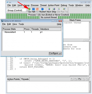
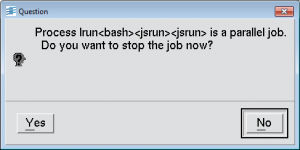

Attaching to a Running Parallel Job
- Find where the job's jsrun job manager process is running. This is usually the first compute node in the job's node list.
- The bquery -X and lsfjobs -v commands can be used to show the job's node list.
- Start totalview on a login node, or else rsh directly to the node where the jobs' jsrun process is running and start totalview there: totalview &
- If you choose to rsh directly to the node, skip to step 5.
- After totalview starts, select "A running program" from the "Start a Debugging Session" dialog window, as shown in (1) below.
- When the "Attach to running program(s)" window appears, click on the H+ button to add the name of the host where the jobs' jsrun process is running. Enter the node's name in the "Add Host" dialog box and click OK, as shown in (2) below.
- After totalview connects to the node, you should see the jsrun process in the process list. Select it, and click "Start Session" as shown in (3) below.
- Totalview will attach to the job and the totalview Root and Process windows will appear to allow you to begin debugging the running job. (click images for larger version)
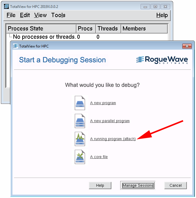
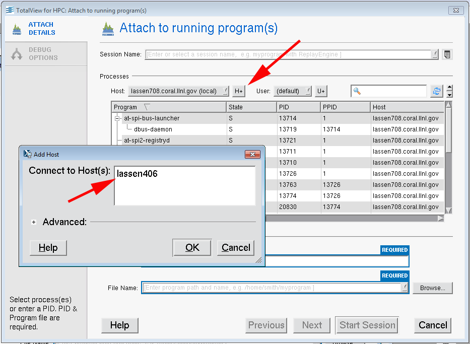
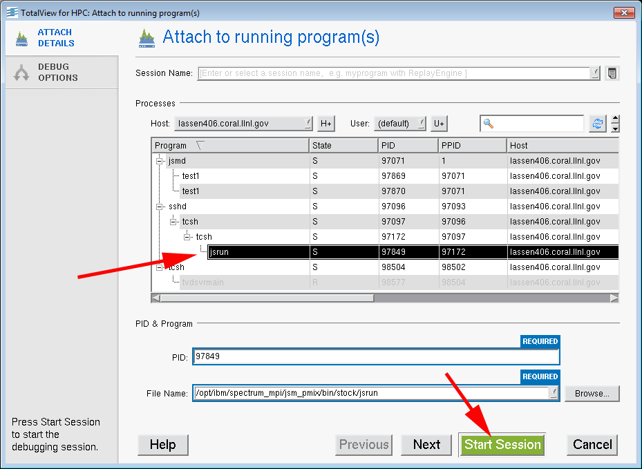
Debugging GPU Code on Sierra
- TotalView supports GPU debugging on Sierra systems:
- CUDA with NVIDIA NVCC compiler
- OpenMP target regions with IBM XL and CLANG compilers
- NVIDIA CUDA recommended compiler options:
- -O0 -g -G -arch sm_60 : to generate GPU DWARF and avoid just-in-time (JIT) compilation for improved performance.
- -dlink : reduce number of GPU ELF images when linking GPU object files into a large image; improves performance.
- IBM XL recommended compiler options:
- -O0 -g -qsmp=omp:noopt -qfullpath -qoffload : generate debug information, no optimization, OpenMP with offloading. Should be sufficient for most applications.
- -qnoinline -Xptxas -O0 -Xllvm2ptx -nvvm-compile-options=-opt=0 : may be necessary for heavily templated codes, or if previous compile options result in "odd" code motion.
- Clang recommended compiler options:
- -fopenmp -fopenmp-targets=nvptx64-nvidia-cuda --cuda-noopt-device-debug : enable OpenMP offloading for NVIDIA GPUs; no optimization with cuda device debug generation.
- For the most part, the basics of running GPU-enabled applications under TotalView are similar to those of running other applications. However, there are unique GPU features and usage details, which are discussed in the "More Information" links below (the TotalView CORAL Update in particular).
More Information
- LC Tutorial: https://hpc.llnl.gov/training/tutorials/totalview-tutorial
- Sierra systems usage notes: https://lc.llnl.gov/confluence/display/SIERRA/TotalView
- TotalView CORAL Update
- Vendor website: https://www.roguewave.com/
STAT
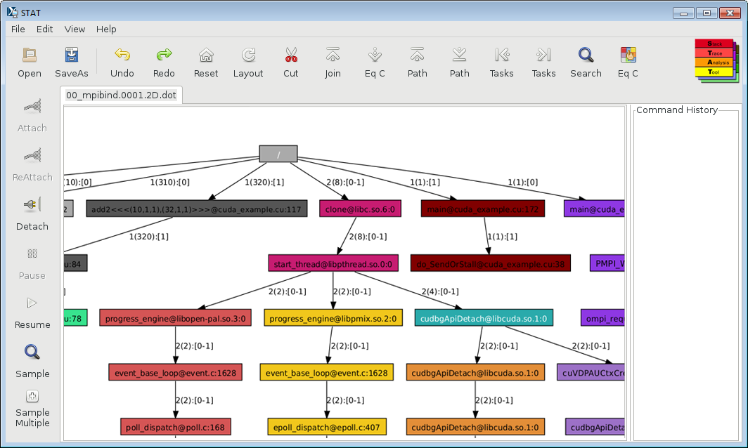
- The Stack Trace Analysis Tool (STAT) gathers and merges stack traces from a parallel application's processes.
- Primarily intended to attach to a hung job, and quickly identify where the job is hung. The output from STAT consists of 2D spatial and 3D spatial-temporal graphs. These graphs encode calling behavior of the application processes in the form of a prefix tree. Example of a STAT 2D spatial graph shown on right (click to enlarge).
- Graph nodes are labeled by function names. The directed edges show the calling sequence from caller to callee and are labeled by the set of tasks that follow that call path. Nodes that are visited by the same set of tasks are assigned the same color.
- STAT is also capable of gathering stack traces with more fine-grained information, such as the program counter or the source file and line number of each frame.
- STAT has demonstrated scalability over 1,000,000 MPI tasks and its logarithmic scaling characteristics position it well for even larger systems.
- STAT is supported on most LC platforms, including Linux, Sierra/CORAL EA, and BG/Q. It works for Message Passing Interface (MPI) applications written in C, C++, and Fortran and supports threads.
- The default version of STAT should be in your path automatically:
- To view all available versions: module avail stat
- To load a different version: module load module_name
- For details on using modules: https://hpc.llnl.gov/software/modules-and-software-packaging.
Quickstart
- Only a brief quickstart summary is provided here - please see the More Information section below for details.
- In a typical usage case, you have already launched a job which appears to be hung. You would then use STAT to debug the job.
- First, find where the job's jsrun job manager process is running. This is usually the first compute node in the job's node list.
The bquery -X and lsfjobs -v commands can be used to show the job's node list. - Start STAT using the stat-gui command on a login node, or else rsh directly to the node where the jobs' jsrun process is running and start stat-gui there.
If you choose to rsh directly to the node, skip to step 5. - Two STAT windows will appear. In the "Attach" window, enter the name of the compute node where your jsrun process is running, and then click "Search Remote Host" as shown in (1) below.
- STAT will then display the jsrun process running on the first compute node. Make sure it is selected and then click "Attach", as shown in (2) below.
-
A 2D graph of your job's merged stack traces will appear, as shown in (3) below. You can now use STAT to begin debugging your job. See the "More Information" section below for links to STAT debugging details. (click images for larger version)
1.)
2.)
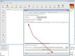
3.)
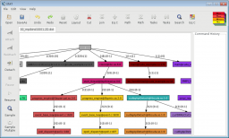
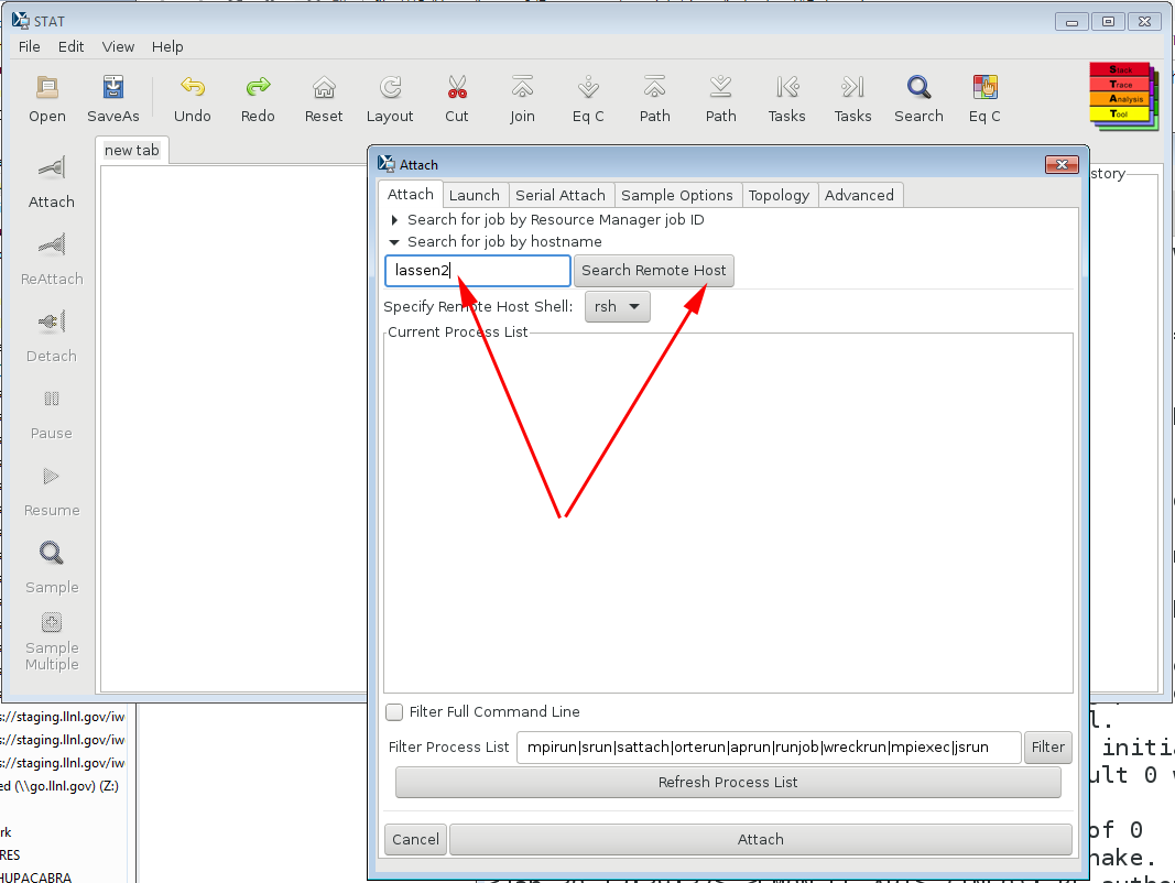
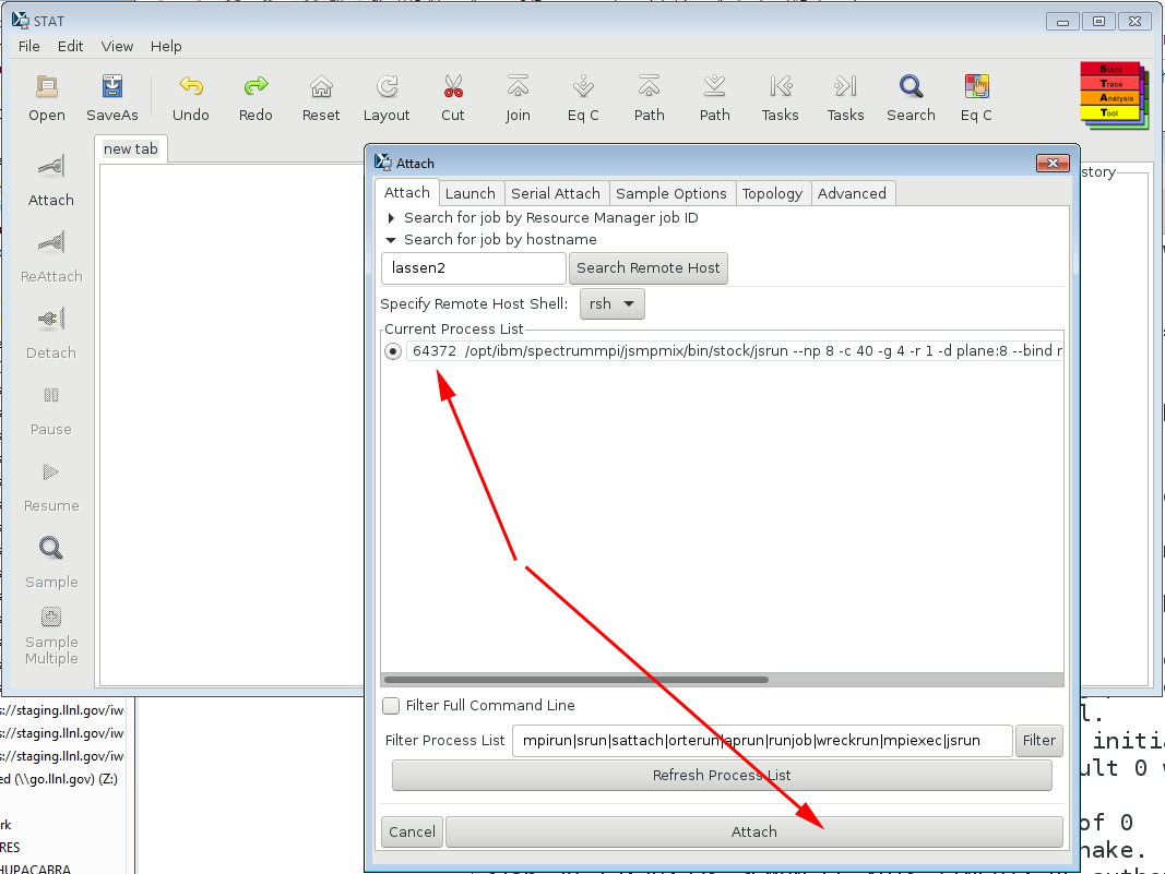
More Information
- STAT User Guide: https://github.com/LLNL/STAT/blob/develop/doc/userguide/stat_userguide.pdf
- LC web pages: https://hpc.llnl.gov/software/development-environment-software/stat-stack-trace-analysis-tool
- Sierra usage notes: https://lc.llnl.gov/confluence/pages/viewpage.action?pageId=544145673 (internal LC wiki)
- STAT man page or help menu: man stat-gui or stat-gui -h (note: you may need to module load stat to get your MANPATH properly set).
Core Files
- TotalView can be used to debug core files. This topic is discussed in detail at: https://hpc.llnl.gov/training/tutorials/totalview-part-2-common-functions#Viewing_a_Core_File.
- For Sierra systems, there are also hooks in place that inform jsrun to dump core files for GPU or CPU exceptions.
- These core files can be full core files or lightweight core files.
-
LC has created options that can be used with the jsrun and lrun commands to specify core file generation and format. Use the --help flag to view. For example:
% jsrun --help

<snip>

LLNL-specific jsrun enhancements from wrapper:
  --core=<format>       Sets both CPU & GPU coredump env vars to <format>
  --core_cpu=<format>   Sets LLNL_COREDUMP_FORMAT_CPU to <format>
  --core_gpu=<format>   Sets LLNL_COREDUMP_FORMAT_GPU to <format>
    where <format> may be core|lwcore|none|core=<mpirank>|lwcore=<mpirank>
  --core_delay=<secs>   Set LLNL_COREDUMP_WAIT_FOR_OTHERS to <secs>
  --core_kill=<target>  Set LLNL_COREDUMP_KILL to <target>
    where <target> may be task|step|job (defaults to task)
% lrun --help <snip> --core=<format> Sets both CPU & GPU coredump env vars to <format> --core_delay=<secs> Set LLNL_COREDUMP_WAIT_FOR_OTHERS to <secs> --core_cpu=<format> Sets LLNL_COREDUMP_FORMAT_CPU to <format> --core_gpu=<format> Sets LLNL_COREDUMP_FORMAT_GPU to <format> where <format> may be core|lwcore|none|core=<mpirank>|lwcore=<mpirank> - LC has also the stat-core-merger utility that can be used to merge and view these core files using STAT.
- For usage information, simply type stat-core-merge
-
Example:
% stat-core-merger -x a.out -c core.*
merging 3 trace files
066%... done!
outputting to file "STAT_merge.dot" ...done!
outputting to file "STAT_merge_1.dot" ...done!
View the outputted .dot files with `STATview`

% stat-view STAT_merge.dot STAT_merge_1.dot
Performance Analysis Tools
For information on available Performance Analysis Tools, please see the following sources:
Development Environment Software: https://hpc.llnl.gov/software/development-environment-software
Code Development Tools on LC's Confluence Wiki: https://lc.llnl.gov/confluence/display/SIERRA/Code+Development+Tools (requires authentication)
Information on using the NIVIDIA nvprof profiler can be found at: https://docs.nvidia.com/cuda/profiler-users-guide .
Information on using the NVIDIA NSIGHT profiling system can be found at: https://docs.nvidia.com/nsight-systems .
Tutorial Evaluation
We welcome your evaluation and comments on this tutorial.
Please complete the online evaluation form
Thank you!
References & Documentation
- Author: Blaise Barney, Lawrence Livermore National Laboratory.
- Ray cluster photos: Randy Wong, Sandia National Laboratories.
- Sierra cluster photos: Adam Bertsch and Meg Epperly, Lawrence Livermore National Laboratory.
Livermore Computing General Documentation
- Livermore Computing user web pages: https://hpc.llnl.gov
- MyLC Livermore Computing user portal: mylc.llnl.gov
- Livermore Computing tutorials: https://hpc.llnl.gov/training/tutorials
CORAL Early Access systems, POWER8, NVIDIA Pascal
- "IBM Power System S822LC for High Performance Computing Introduction and Technical Overview" IBM Redpaper publication REDP-5405-00 by Alexandre Bicas Caldeira, Volker Haug, Scott Vetter. September, 2016.
- "NVIDIA Tesla P100". NVIDIA Whitepaper. 2016.
- NVIDIA CUDA Toolkit documentation
- CORAL Early Access systems user information (internal LC wiki): https://lc.llnl.gov/confluence/display/CORALEA/CORAL+EA+Systems
Sierra systems, POWER9, NVIDIA Volta
- IBM Power System AC922 Introduction and Technical Overview. IBM Redbook publication REDP-5472-00 by Alexandre Bicas Caldeira. March 2018.
- "Implementing an IBM High-Performance Computing Solution on IBM Power System S822LC". IBM Redbook publication SG24-8280-00. July 2016.
- "NVIDIA Tesla V100 GPU Architecture". NVIDIA Whitepaper. August 2017.
- NVIDIA CUDA Toolkit documentation
- Sierra systems user information (internal LC wiki): https://lc.llnl.gov/confluence/display/SIERRA/Sierra+Systems
LSF Documentation
- IBM Spectrum LSF online documentation
- IBM Knowledge Center LSF documentation
- LC's LSF documents located at: https://hpc.llnl.gov/banks-jobs/running-jobs
Compilers and MPI Documentation
- XLC/C++: Select the relevant version of Little Endian documents at https://www-01.ibm.com/support/docview.wss?uid=swg27036675
- XLF: Select the relevant version of Little Endian documents at https://www-01.ibm.com/support/docview.wss?uid=swg27036672
- IBM White Paper "Code Optimization with the IBM XL compilers on Power Architectures": https://www-01.ibm.com/support/docview.wss?uid=swg27005174&aid=1
- IBM MPI Spectrum Documentation at: https://www.ibm.com/docs/en/spectrum-lsf/10.1.0
Quick start guide, release notes, installation, user guide and more. - GNU compiler online documentation at: https://gcc.gnu.org/onlinedocs/
- PGI Compilers: https://docs.nvidia.com/hpc-sdk/pgi-compilers/19.1/x86/pgi-ref-guide/in…
Appendix A: Quickstart Guide
This section provides both a "Lightning-quick" and "Detailed" Quickstart Guide. For more information, see the relevant sections in the full tutorial.
Lightning-quick Quickstart Guide
- If you cannot find what you need on these pages, the LC Hotline <lc-hotline@llnl.gov>, 925-422-4531, can help!
- Use lsfjobs to find the state of the job queue.
- Use news job.lim.<machinename> to see the job queue limits for a machine. For example on sierra: news job.lim.sierra
- Use lalloc <number of nodes> to get an interactive allocation and a shell on the first allocated compute node. For example, allocate 2 nodes for 30 minutes in the pdebug queue:
lalloc 2 -W 30 -q pdebug - Use bsub -nnodes <number of nodes> myscript to run a batch job script on the first allocated compute node
- Query your bank usage with command: lshare -u <user_name> on Lassen or Sierra (not on Rzansel, Ray, Rzmanta or Shark)
- Always build with and use the default MPI (spectrum-mpi/rolling-release) unless specifically told otherwise.
- Running jobs using lrun is recommended (but jsrun and the srun emulator are the other options): Syntax:
lrun -n <ntasks>|-T <ntasks_per_node> [-N <nnodes>] [ many more options] <app> [app-args] - Run lrun with no args for detailed help. Add -v to see the jsrun invocation that lrun generates.
- The easy way to use lrun is to specify tasks per node with the -T option and let lrun figure out the number of ranks from the allocation. For example: lrun -T4 hello.exe will run 4 ranks in a 1 node allocation and 16 tasks evenly distributed on a 4 node allocation
- lrun -T1 hostname | sort gets you the list of nodes you were allocated
- Use the -M "-gpu" option to use GPUDirect with device or managed memory buffers. No CUDA API calls (including cudaMallocManaged) are permitted before the MPI_Init call or you may get the wrong answer!
- Don't build big codes on a login or launch node (basically don't slam any node with other users on it). Use bsub or lalloc to get a dedicated compute node before running make -j.
- The -m "launch_hosts sierra24" option of bsub requests a particular node or nodes (compute node sierra24 in this case)
- To submit a 2048 node job to the pbatch queue with core isolation and 4 ranks per node for 24 hours:
bsub -nnodes 2048 -W 24:00 -G pbronze -core_isolation 2 -q pbatch lrun -T4 <executable> <args> - You can check your node(s) using check_sierra_nodes (but you are unlikely to find bad nodes at this point)
- Use lrun --smt=4 <options> to use 4 hardware threads per core.
Detailed Quickstart Guide
Table of Contents
- How to get help from an actual human
- If direct ssh to LASSEN or SIERRA fails, login from somewhere inside LLNL first
- First time LASSEN/SIERRA/RZANSEL users should verify their default bank and ssh key setup first
- Use lsfjobs to see machine state
Use news job.lim.<machinename> to see queue limits - Allocate interactive nodes with lalloc
- Known issue running on the first backend compute node (12 second X11 GUI startup, Error initializing RM connection, --stdio_stderr --stdio_stdout broken)
- How to start a 'batch xterm' on CORAL
- Disabling core isolation with bsub -core_isolation 0 (and the one minute node state change)
- The occasional one minute bsub startup and up to five minute bsub teardown times seen in lsfjobs output
- Batch scripts with bsub and a useful bsub scripts trick
- How to run directly on the shared batch launch node instead of the first compute node
- Should MPI jobs be launched with lrun, jsrun, the srun emulator, mpirun, or flux?
- Running MPI jobs with lrun (recommended)
- Examples of using lrun to run MPI jobs
- How to see which compute nodes you were allocated
- CUDA-aware MPI and Using Managed Memory MPI buffers
- MPI Collective Performance Tuning
1. How to get help from an actual human
If something is not working right on any machine (CORAL or otherwise), your best bet is to contact the Livermore Computing Hotline, Hours: M-F: 8A-12P,1-4:45P, Email: lc-hotline@llnl.gov, Phone: 925-422-4531. For those rare CORAL error messages that ask you to contact the Sierra development environment point of contact John Gyllenhaal (gyllen@llnl.gov, (925) 424-5485), please contact John Gyllenhaal and also cc the LC Hotline to track the issues.
2. If direct ssh to LASSEN or SIERRA fails, login from somewhere inside LLNL first
We believe you can now login directly to LASSEN (from the internet) and SIERRA (on the SCF network) but if that does not work, tell us! A workaround is to login to oslic (for LASSEN) or cslic (for SIERRA) first. As of Aug 2019, RZANSEL can be accessed directly without the need to go through rzgw.llnl.gov first. LANL and Sandia users should start from an iHPC node. Authentication is with your LLNL username and RZ PIN + Token.
3. First time LASSEN/SIERRA/RZANSEL users should verify their default bank and ssh key setup first
The two issues new CORAL users typically encounter are 1) not having a compute bank set up or 2) having incompatible ssh keys copied from another machine. Running the following lalloc command (with a short time limit to allow fast scheduling) will check both and verify you can run an MPI job:
$ lalloc 1 -W 3 check_sierra_nodes
<potentially a bunch of messages about setting up your ssh keys>
+ exec bsub -nnodes 1 -W 3 -Is -XF -core_isolation 2 /usr/tce/packages/lalloc/lalloc-2.0/bin/lexec check_sierra_nodes
Job <389127> is submitted to default queue <pbatch>.
<<ssh X11 forwarding job>>
<<Waiting for dispatch ...>>   <--This indicates have bank and ssh keys setup correctly, can hit Control-C if machine really busy
<<Starting on lassen710>>
<<Waiting for JSM to become ready ...>>
<<Redirecting to compute node lassen449, setting up as private launch node>>
STARTED: 'jsrun -r 1 -g 4 test_sierra_node -mpi -q' at Mon Jul 22 14:19:42 PDT 2019
SUCCESS: Returned 0 (all, including MPI, tests passed) at Mon Jul 22 14:19:46 PDT 2019  <--MPI worked for you, you are all set!
logout
If you don't have a compute bank set up, you will get a message to contact your computer coordinator:
+ exec bsub -nnodes 1 -Is -W 60 -core_isolation 2 /usr/tce/packages/lalloc/lalloc-2.0/bin/lexec
You do not have a default group (bank). <--This indicates bank PROBLEM
Please specify a bank with -G option or contact your computer coordinator to request a bank.
A list of computer coordinators is available at https://myconfluence.llnl.gov/pages/viewpage.action?spaceKey=HPCINT&title=Computer+Coordinators
or through the "my info" portlet at https://lc.llnl.gov/lorenz/mylc/mylc.cgi
Request aborted by esub. Job not submitted.
If you have passphrases on your ssh keys, you will see something like:
==> Ah ha! ~/.ssh/id_rsa encrypted with passphrase, likely the problem!
    Highly recommend using passphrase-less keys on LC to minimize issues

Error: Passphrase-less ssh keys not set up properly for LC CORAL clusters  <--This indicates ssh keys PROBLEM
       You can remove an existing passphrase by running 'ssh-keygen -p',
         selecting your ssh key (i.e., .ssh/id_rsa), entering your current passphrase,
         and hitting enter for your new passphrase.
       lalloc/lrun/bsub/jsrun will likely fail with mysterious errors
Typically removing an existing passphrase by running ssh-keygen -p, selecting your ssh key (i.e., .ssh/id_rsa), entering your current passphrase, and hitting enter for your new passphrase will solve the problem. Otherwise contact John Gyllenhaal (gyllen@llnl.gov, 4-5485) and cc the LC Hotline lc-hotline@llnl.gov for help with ssh key setup. Having complicated .ssh/config setups can also break ssh keys.
4. Use lsfjobs to see machine state
Use news job.lim.<machinename> to see queue limits
Use the lsfjobs command to see what is running, what is queued and what is available on the machine. See the lsfjobs section for details.
sierra4368$  lsfjobs
<snip>
*******************************************************************************************************
* QUEUE           NODE GROUP      Total   Down    Busy   Free  NODES                                  *
*******************************************************************************************************
   -               debug_hosts        36      1       0     35  sierra[361-396]
   -               batch_hosts       871     14     212    645  sierra[397-531,533-612,631-684,703-720,1081-1170,1189-1440,1819-2060]
<snip>
As with all LC clusters, you can quickly view the job queue limits for a given machine by using the command news job.lim.<machinename>. For example, on sierra: news job.lim.sierra.
Queue limits are also available on the web via the MyLC Portal:
- mylc.llnl.gov
- Click on a machine name in the "machine status" portlet, or the "my accounts" portlet.
- Then select the "details", "topology" and/or "job limits" tabs for detailed hardware and configuration information.
Common queue limits include the maximum number of nodes, maximum time limit, maximum number of running jobs, etc. Limits are subject to change, and are different for every cluster.
5. Allocate interactive nodes with lalloc
Use the LLNL-specific lalloc bsub wrapper script to facilitate interactive allocations on CORAL and CORAL EA systems. The first and only required argument is the number of nodes you want followed by optional bsub arguments to pick queue, length of the allocation, etc. Note By default, all Sierra systems and CORAL EA systems use lalloc/2.0, which uses 'lexec' to place the shell for the interactive allocation on the first compute node of the allocation.
The lalloc script prints out the exact bsub line used. For example, 'lalloc 2' will give you 2 nodes with those listed defaults:
lassen708{gyllen}2: lalloc 2
+ exec bsub -nnodes 2 -Is -XF -W 60 -G guests -core_isolation 2 /usr/tce/packages/lalloc/lalloc-2.0/bin/lexec
Job <3564> is submitted to default queue <pbatch>.
<<ssh X11 forwarding job>>
<<Waiting for dispatch ...>>
<<Starting on lassen710>>
<<Redirecting to compute node lassen90, setting up as private launch node>>
Run 'lalloc' with no arguments for usage info. Here is the current usage info for lalloc/2.0 as of 7/19/19:
Usage: lalloc #nodes <--shared-launch> <--quiet> <supported bsub opts> <command>
Allocates nodes interactively on LLNL's CORAL and CORAL EA systems
and executes a shell, or the optional <command>, on the first compute node
(which is set up as a private launch node) instead of a shared launch node

lalloc specific options:
--shared-launch Use shared launch node instead of a private launch node
--quiet Suppress bsub and lalloc output (except on errors)

Supported bsub options:
-W minutes Allocation time in minutes (default: 60)
-q queue Queue to use (default: system default queue)
-core_isolation # Cores per socket used for system processes (default: 2)
-G group Bsub fairshare scheduling group (former default: guests)
-Is|-Ip|-I<x> Interactive job mode (default: -Is)
-XF X11 forwarding (default if DISPLAY set)
-stage "bb_opts" Burst buffer options such as "storage=2"
-U reservation Bsub reservation name

Example usage:
lalloc 2 (Gives interactive shell with 2 nodes and above defaults)
lalloc 1 make -j (Run parallel make on private launch node)
lalloc 4 -W 360 -q pbatch lrun -n 8 ./parallel_app -o run.out

Please report issues or missing bsub options you need supported to
John Gyllenhaal (gyllen@llnl.gov, 4-5485)
6. Known issue running on the first backend compute node (12 second X11 GUI startup, Error initializing RM connection, --stdio_stderr --stdio_stdout broken)
As of Aug 2019, there are three known issues with running on the first backend node (the new default for bsub and lalloc). One workaround is to use --shared-launch to land on the shared launch node (but please don't slam this node with builds, etc.).
1) Some MPI errors cause allocation daemons to die, preventing future lrun/jsrun invocations from working (gives messages like: Could not find the contact information for the JSM daemon. and: Error initializing RM connection. Exiting.). You must exit the lalloc shell and do another lalloc to get a working allocation. As of February 2019, this is a much rarer problem but we still get some reports of issues when hitting Control-C. Several fixes for these problems are expected in the September 2019 update.
2) The lrun/jsrun options --stdio_stderr --stdio_stdout options don't work at all on the backend nodes. Either don't use them or use --shared-launch to run lrun and jsrun on the launch node. Expected to be fixed in September 2019 update.
3) Many X11 GUI programs (gvim, memcheckview, etc.) have a 12 second delay the first time they are invoked. Future invocations in the same allocation work fine. Sometimes, the allocation doesn't exit properly after typing 'exit' until control-C is hit. This is caused the startup of dbus-daemon, which is commonly used by graphics programs. We are still exploring solutions to this.
7. How to start a 'batch xterm' on CORAL
You can run commands interactively with lalloc (like xterm) and you can make lalloc silent with the --quiet option. So an easy way to start a 'batch xterm' is:
lalloc 1 -W 60 --quiet xterm -sb &
Your allocation will go away when the xterm is exited. Your xterm will go away when the allocation ends.
8. Disabling core isolation with bsub -core_isolation 0 (and the one minute node state change)
As of February 2019, '-core_isolation 2' is the default behavior if -core_isolation is not specified on the bsub line. This isolates all the system processes (including GPFS daemons) to 4 cores per node (2 per socket). With 4 cores per node dedicated for system processes, we believe there should be relatively little impact on GPFS performance (except perhaps if you are running the ior benchmark). You may explicitly disable core isolation by specifying '-core_isolation 0' on the bsub or lalloc line but we don't recommend it .
9. The occasional one minute bsub startup and up to five minute bsub teardown times seen in lsfjobs output
When bsub allocation starts (lsfjobs shows state as 'running'), the core_isolation mode state is checked against the requested mode. If the node modes are different, it takes about 1 minute to set up the nodes(s) in the new core_isolation mode. So if the previous user of one or nodes used a different core_isolation setting than your run, you will get a mysterious 1 minute delay before your job actually starts running. This is why we recommend everyone stay with the default -core_isolation 2 setting.
After the bsub allocation ends, we run more than 50 node health checks before returning the node for use in a new allocation. These tests require all running user processes to terminate first and if the user processes are writing to disk over the network, it sometimes takes a few minutes for them to terminate. We have a 5 minute timeout waiting for tasks to end before we give up and drain the node for a sysadmin to look at. This is why it is not uncommon to have to wait 15 to 120 seconds before all the nodes for an allocation are actually released.
10. Batch scripts with bsub and a useful bsub scripts trick
The only way to submit batch jobs is 'bsub'. You may specify a bsub script at the end of the bsub command line, put a full command on the end of the bsub command line, or pipe a bsub script into stdin. As of June 2019 (on LASSEN and RZANSEL only), this script will run on the first compute node of your allocation (see next section for more details).
For example, a batch shell script can be submitted via:
bsub -nnodes 32 -W 360 myapp.bsub
or equivalently
bsub -nnodes 32 -W 360 < myapp.bsub
In both cases, additional bsub options may be specified in the script via one or more '#BSUB <list of bsub options>' lines.
It is often useful to have a script that submits bsub scripts for you. It is often convenient to use the 'cat << EOF' trick to embed the bsub script you wish to pipe in to stdin in your script. Here is an example of this technique:
sierra4359{gyllen}52: cat do_simple_bsub
#!/bin/sh
cat << EOF | bsub -nnodes 32 -W 360
#!/bin/bash <-- optionally set shell language, bash default
#BSUB -core_isolation 2 -G guests -J "MYJOB1"
cd ~/debug/hasgpu
lrun -T 4 ./mpihasgpu arg1 arg2
EOF

sierra4359{gyllen}53: ./do_simple_bsub
Job <143505> is submitted to default queue .
11. How to run directly on the shared batch launch node instead of the first compute node
As of June 2019, LASSEN's and RZANSEL's bsub by default runs your bsub script on the first compute node (like SLURM does), to prevent users from accidentally slamming and crashing the shared launch node. Although it is no longer the default behavior, you are welcome to continue to use the shared launch node to launch jobs (but please don't build huge codes on the shared launch node or the login nodes). To get access back to the shared launch node, use the new LLNL-specific option '--shared-launch' with either bsub or lalloc. To force the use of the first compute node, use '--private-launch' with either bsub or lalloc.
12. Should MPI jobs be launched with lrun, jsrun, the srun emulator, mpirun, or flux?
The CORAL contract required IBM to develop a new job launcher (jsrun) with a long list of powerful new features to support running regression tests, UQ runs, and very complex job launch configurations that was missing in SLURM's srun, the job launcher on all of LLNL's other supercomputers. IBM's jsrun delivered all the power we required at the cost of a more complex interface that is very different than the interface for SLURM's srun. This more complex jsrun interface makes a lot of sense if you need all of its power (and the complexity is unavoidable), but many of our user's use cases do not need all this power. For this reason, 'lrun' was written by LLNL as a wrapper over jsrun to provide an srun-like interface to jsrun that captures perhaps 95% of the use cases. Later, LLNL wrote a 'srun' emulator that provides an exact srun interface (for a common subset of srun options) that captures perhaps 80% of the our user's use cases (and uses lrun and thus jsrun under the covers). In parallel, LLNL also developed flux, a powerful new job scheduler that has a different portable solution for all those features missing in SLURM and it can run on all LLNL supercomputers. Lastly, the old 'mpirun' command still exists but is mostly broken and should be not be used unless you have a truly compelling need to do so .
Recommendations:
Use 'lrun' for almost all use cases. It does very good default binding and layout of runs, including for regression tests (use the --pack, -c, and -g options) and UQ (use the -N option) runs. The lrun command defaults to a node-schedule mode (unless --pack option used), unlike jsrun and srun, so simultaneous job steps will not share nodes by default (which is typically what you want for UQ). In '--pack' mode (regression test mode), uses jsrun's enhanced binding algorithm (designed for regression tests) instead of mpibind.
Use 'jsrun' only if you need complete control of MPI task placement/resources or if you want to run the same bsub script on ORNL's SUMMIT cluster (or other non-LLNL CORAL clusters). The jsrun command defaults to core-scheduled mode (like srun does), so concurrent jobs will shared nodes unless the specified resource constraints prevent it.
Use flux (contact the flux team) if you want a regression test or UQ solution that can run on all LLNL supercomputers, not just CORAL. The 'flux' system has a scalable python interface for submitting a large number of jobs with exactly the layout desired that is portable to all LLNL machines (and eventually all schedulers).
Use 'srun' if you want an actual srun interface for regression tests or straightforward one-at-a-time runs. Not a good match for UQ runs (non-trivial to prevent overlapping simultaneous job steps on the same node) and srun will punt if you use an unsupported options (emulator does not support manual placement options, use jsrun for that). The srun command defaults to core-scheduled mode and using mpibind (uses lrun with --pack --mpibind=on by default), so simultaneous job steps will share nodes by default.
Do NOT use 'mpirun' unless one of the above solutions does not work and you really know what you are doing (takes > 100 character of options to make mpirun work right on CORAL and not crash the machine). Some science run users use mpirun combined with flux, so mpirun is allowed on compute nodes but will not run by default on login or launch nodes.
13. Running MPI jobs with 'lrun' (recommended)
In most cases (as detailed above) we recommend you use the LC-written 'lrun' wrapper for jsrun, instead of using jsrun directly to launch jobs on the backend compute nodes. By default, lrun uses node-scheduling (job steps will not share nodes) unlike jsrun or the srun emulator, which is good for single runs and UQ runs. If you wish to run multiple simultaneous job steps on the same nodes for regression tests, use the --pack option and specify cpus-per-task and gpus-per-task with -c and -g. If you wish to use multiple threads per core, use the --smt option or specify the desired number of threads with OMP_NUM_THREADS. Running lrun no arguments will give the following help text (as of July 2019):
Usage: lrun -n <ntasks> | -T <ntasks_per_node> | -1 \
[-N <nnodes>] [--adv_map] [--threads=<nthreads>] [--smt=<1|2|3|4>] \
[--pack] [-c <ncores_per_task>] [-g <ngpus_per_task>] \
[-W <time_limit> [--bind=off] [--mpibind=off|on] [--gpubind=off] \
[--core=<format>] [--core_delay=<secs>] \
[--core_gpu=<format>] [--core_cpu=<format>] \
[-X <0|1>] [-v] [-vvv] [<compatible_jsrun_options>] \
<app> [app-args]

Launches a job step in a LSF node allocation with a srun-like interface.
By default the resources for the entire node are evenly spread among MPI tasks.
Note: for 1 task/node, only one socket is bound to unless --bind=off used.
Multiple simultaneous job steps may now be run in allocation for UQ, etc.
Job steps can be packed tightly into nodes with --pack for regression testing.

AT LEAST ONE OF THESE LRUN ARGUMENTS MUST BE SPECIFIED FOR EACH JOB STEP:
-n <ntasks> Exact number of MPI tasks to launch
-T <ntasks_per_node> Layout ntasks/node and if no -n arg, use to calc ntasks
-1 Run serial job on backend node (e.g. lrun -1 make)
-1 expands to '-N 1 -n 1 -X 0 --mpibind=off'

OPTIONAL LRUN ARGUMENTS:
-N <nnodes> Use nnodes nodes of allocation (default use all nodes)
--adv_map Improved mapping but simultaneous runs may be serialized
--threads=<nthreads> Sets env var OMP_NUM_THREADS to nthreads
--smt=<1|2|3|4> Set smt level (default 1), OMP_NUM_THREADS overrides
--pack Pack nodes with job steps (defaults to -c 1 -g 0)
--mpibind=on Force use mpibind in --pack mode instead of jsrun's bind
-c <ncores_per_task> Required COREs per MPI task (--pack uses for placement)
-g <ngpus_per_task> Required GPUs per MPI task (--pack uses for placement)
-W <time_limit> Sends SIGTERM to jsrun after minutes or H:M or H:M:S
--bind=off No binding/mpibind used in default or --pack mode
--mpibind=off Do not use mpibind (disables binding in default mode)
--gpubind=off Mpibind binds only cores (CUDA_VISIBLE_DEVICES unset)
--core=<format> Sets both CPU & GPU coredump env vars to <format>
--core_delay=<secs> Set LLNL_COREDUMP_WAIT_FOR_OTHERS to <secs>
--core_cpu=<format> Sets LLNL_COREDUMP_FORMAT_CPU to <format>
--core_gpu=<format> Sets LLNL_COREDUMP_FORMAT_GPU to <format>
where <format> may be core|lwcore|none|core=<mpirank>|lwcore=<mpirank>
-X <0|1> Sets --exit_on_error to 0|1 (default 1)
-v Verbose mode, show jsrun command and any set env vars
-vvv Makes jsrun wrapper verbose also (core dump settings)

JSRUN OPTIONS INCOMPATIBLE WITH LRUN (others should be compatible):
-a, -r, -m, -l, -K, -d, -J (and long versions like --tasks_per_rs, --nrs)
Note: -n, -c, -g redefined to have different behavior than jsrun's version.

ENVIRONMENT VARIABLES THAT LRUN/MPIBIND LOOKS AT IF SET:
MPIBIND_EXE <path> Sets mpibind used by lrun, defaults to:
/usr/tce/packages/lrun/lrun-2019.05.07/bin/mpibind10
OMP_NUM_THREADS # If not set, mpibind maximizes based on smt and cores
OMP_PROC_BIND <mode> Defaults to 'spread' unless set to 'close' or 'master'
MPIBIND <j|jj|jjj> Sets verbosity level, more j's -> more output

Spaces are optional in single character options (i.e., -T4 or -T 4 valid)
Example invocation: lrun -T4 js_task_info

Written by Edgar Leon and John Gyllenhaal at LLNL.
Please report problems to John Gyllenhaal (gyllen@llnl.gov, 4-5485)
14. Examples of using lrun to run MPI jobs
JSM includes the utility program 'js_task_info' that provides great binding and mapping info, but it is quite verbose. Much of the output below is replaced with '...' for readability.
If you have a 16 node allocation, you can restrict the nodes lrun uses with the -N <nodes> option, for example, on one node:
$ lrun -N 1 -n 4 js_task_info | & sort
Task 0 ... cpu[s] 0,4,... on host sierra1301 with OMP_NUM_THREADS=10 and with OMP_PLACES={0},{4},... and CUDA_VISIBLE_DEVICES=0
Task 1 ... cpu[s] 40,44,... on host sierra1301 with OMP_NUM_THREADS=10 and with OMP_PLACES={40},{44},... and CUDA_VISIBLE_DEVICES=1
Task 2 ... cpu[s] 88,92,... on host sierra1301 with OMP_NUM_THREADS=10 and with OMP_PLACES={88},{92},... and CUDA_VISIBLE_DEVICES=2
Task 3 ... cpu[s] 128,132,... on host sierra1301 with OMP_NUM_THREADS=10 and with OMP_PLACES={128},{132},... and CUDA_VISIBLE_DEVICES=3
All these examples do binding, since --nolbind was not specified.
$ lrun -N 3 -n 6 js_task_info | & sort
Task 0 ... cpu[s] 0,4,... on host sierra1301 with OMP_NUM_THREADS=20 and with OMP_PLACES={0},{4},... and CUDA_VISIBLE_DEVICES=0 1
Task 1 ... cpu[s] 88,92,... on host sierra1301 with OMP_NUM_THREADS=20 and with OMP_PLACES={88},{92},... and CUDA_VISIBLE_DEVICES=2 3
Task 2 ... cpu[s] 0,4,... on host sierra1302 with OMP_NUM_THREADS=20 and with OMP_PLACES={0},{4},... and CUDA_VISIBLE_DEVICES=0 1
Task 3 ... cpu[s] 88,92,... on host sierra1302 with OMP_NUM_THREADS=20 and with OMP_PLACES={88},{92},... and CUDA_VISIBLE_DEVICES=2 3
Task 4 ... cpu[s] 0,4,... on host sierra1303 with OMP_NUM_THREADS=20 and with OMP_PLACES={0},{4},... and CUDA_VISIBLE_DEVICES=0 1
|Task 5 ... cpu[s] 88,92,... on host sierra1303 with OMP_NUM_THREADS=20 and with OMP_PLACES={88},{92},... and CUDA_VISIBLE_DEVICES=2 3
If you don’t specify -N<nodes>, it will spread things across your whole allocation, unlike the default behavior for jsrun:
$ lrun -p6 js_task_info | sort
You can specify -T <tasks_per_nodes> instead of -p<tasks>:
$ lrun -N2 -T4 js_task_info | sort
15. How to see which compute nodes you were allocated
See what compute nodes you were actually allocated using lrun -T1 :
$ lrun -T1 hostname | sort
sierra361
sierra362
<snip>
NOTE: To ssh to the first backend node, use 'lexec'. Sshing directly does not set up your environment properly for running lrun or jsrun.
16. CUDA-aware MPI and Using Managed Memory MPI buffers
CUDA-aware MPI allows GPU buffers (allocated with cudaMalloc) to be used directly in MPI calls. Without CUDA-Aware MPI data must be copied manually to/from a CPU buffer (using cudaMemcpy) before/after passing data in MPI calls. For example:
Without CUDA-aware MPI - need to copy data between GPU and CPU memory before/after MPI send/receive operations.
//MPI rank 0

cudaMemcpy(sendbuf_h,sendbuf_d,size,cudaMemcpyDeviceToHost);
MPI_Send(sendbuf_h,size,MPI_CHAR,1,tag,MPI_COMM_WORLD);

//MPI rank 1
MPI_Recv(recbuf_h,size,MPI_CHAR,0,tag,MPI_COMM_WORLD, &status);
cudaMemcpy(recbuf_d,recbuf_h,size,cudaMemcpyHostToDevice);
With CUDA-aware MPI - data is transferred directly to/from GPU memory by MPI send/receive operations.
With CUDA-aware MPI - data is transferred directly to/from GPU memory by MPI send/receive operations.
//MPI rank 0
MPI_Send(sendbuf_d,size,MPI_CHAR,1,tag,MPI_COMM_WORLD);

//MPI rank 1
MPI_Recv(recbuf_d,size,MPI_CHAR,0,tag,MPI_COMM_WORLD, &status);
IBM Spectrum MPI on CORAL systems is CUDA-aware. However, users are required to "turn on" this feature using a run-time flag with lrun or jsrun. For example:
lrun -M "-gpu"
jsrun -M "-gpu"
Caveat: Do NOT use the MPIX_Query_cuda_support() routine or the preprocessor constant MPIX_CUDA_AWARE_SUPPORT to determine if MPI is CUDA-aware. IBM Spectrum MPI will always return false.
Additional Information:
An Introduction to CUDA-Aware MPI: https://devblogs.nvidia.com/introduction-cuda-aware-mpi/
MPI Status Updates and Performance Suggestions: 2019.05.09.MPI_UpdatesPerformance.Karlin.pdf
17. MPI Collective Performance Tuning
MPI collective performance on sierra may be improved by using the Mellanox HCOLL and SHARP functionality, both of which are now enabled by default. Current benchmarking indicates that using HCOLL can reduce collective latency 10-50% for message sizes larger than 2KiB, while using SHARP can reduce collective latency 50-66% for message sizes up to 2 KiB. Best performance is observed when using both HCOLL and SHARP. As of Aug 2018, we believe we do the below by default for users but the mpiP info below may be useful for tuning parameters further for your application.
- To enable HCOLL functionality, pass the following flags to your jsrun command:
-M "-mca coll_hcoll_enable 1 -mca coll_hcoll_np 0 -mca coll ^basic -mca coll ^ibm -HCOLL -FCA" - To enable SHARP functionality, also pass the following flags to your jsrun command:
-E HCOLL_SHARP_NP=2 -E HCOLL_ENABLE_SHARP=2 - If you wish ensure that SHARP is being used by your job, set the HCOLL_ENABLE_SHARP environment variable to 3, and your job will fail if it cannot use SHARP. Your job will generate messages similar to:
[sierra2545:94746:43][common_sharp.c:292:comm_sharp_coll_init] SHArP: Fallback is disabled. exiting ... - If you wish to generate SHARP log data indicating SHARP statistics and confirming that SHARP is being used, add -E SHARP_COLL_LOG_LEVEL=3. This will generate log data similar to:
INFO job (ID: 4456568) resource request quota: ( osts:64 user_data_per_ost:256 max_groups:0 max_qps:176 max_group_channels:1, num_trees:1)
To determine MPI collective message sizes used by an application, you can use the mpiP MPI profiler to get collective communicator and message size histogram data. To do this using the IBM-provided mpiP library, do the following:
- Load the mpip module with "module load mpip".
- Set the MPIP environment variable to "-y".
- Run your application with lrun-mpip instead of lrun.
- Your application should create an *.mpiP report file with an "Aggregate Collective Time" section with collective MPI Time %, Communicator size, and message size.
- Do not link with "-lmpiP" as this will link with the currently broken IBM mpiP library (as of 10/11/18).
Additional HCOLL environment variables can be found by running "/opt/mellanox/hcoll/bin/hcoll_info --all". Additional SHARP environment variables can be found here.
LLNL-WEB-750771 test